Photon Counting is an acquisition mode suited for extreme faint-flux imaging. Taking full advantage of the EMCCD’s unique sensitivity, photon counting allows to image signals down to a scarce few photons per hour with a single-photon resolution power and a wide field of view.
When signals are under 1 photon/pixel/frame, photon counting is the best option available and has the potential to significantly improve acquisitions, all with remarkable ease of use.
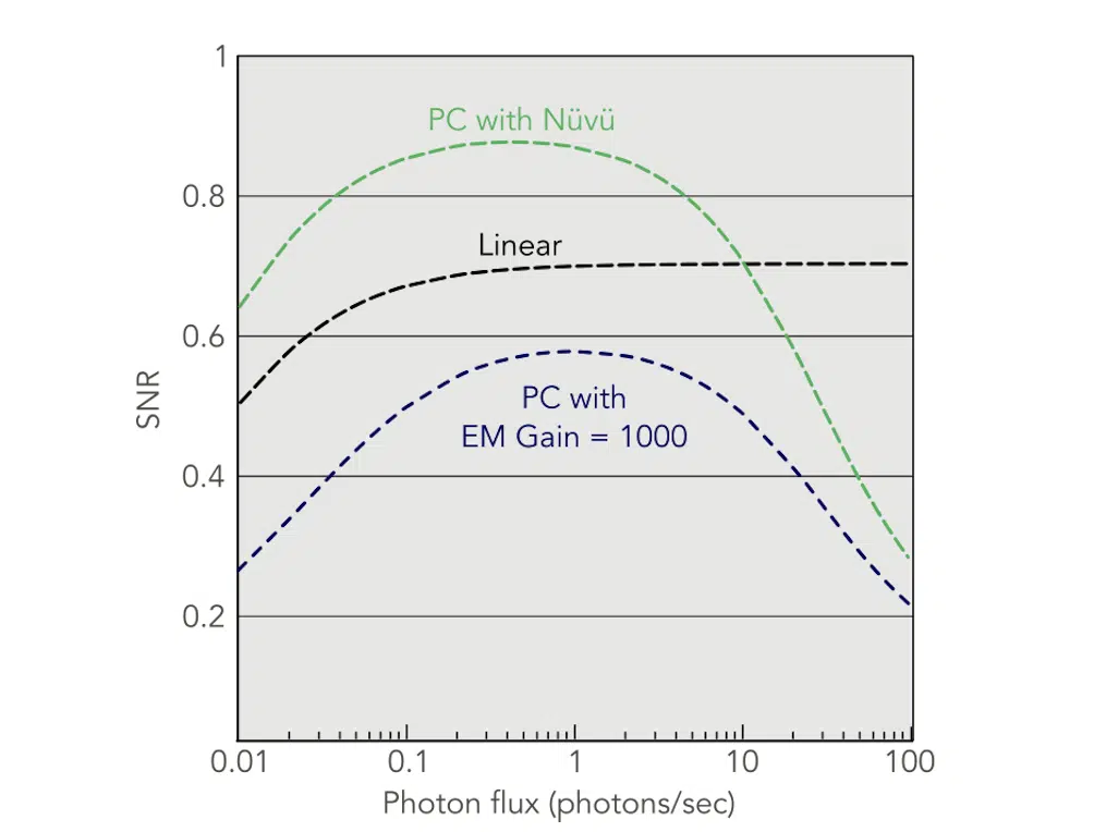
Chief among the reasons to use photon counting (PC) is its increased sensitivity compared to typical linear EMCCD acquisitions (linear mode – LM). All imaging technologies using gain (e.g. avalanche diodes, EMCCD detectors) suffer from what is called the excess noise factor (ENF). Gain is a stochastic process and electrons have a certain probability to be multiplied at each stage of the multiplication register so even for a set gain, there is a pixel by pixel uncertainty on the exact number of electrons at the output of multiplication. The ENF is a representation of this phenomenon and has the same effect on the signal-to-noise ratio (SNR) as dividing your camera’s quantum efficiency in half. More details on this subject are available in EMCCD noise sources.
Using photon counting eliminates the effect of ENF; the same impact as multiplying your signal two-fold. This increased sensitivity makes a crucial difference when imaging low signal levels.
It can be observed that the benefits of photon counting do not extend beyond a signal of 1 photon/pixel/frame. That is because photon counting produces binary images, with each pixel either being a 0, where no photon was detected, and 1, where a photon was detected. As such, if a pixel receives more than 1 photon, this information is not registered by the image which results in a coincidence loss.
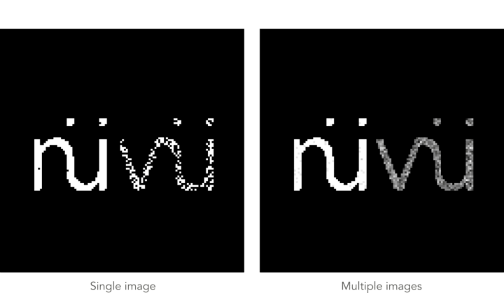
While a single photon counting image is binary, multiple images can be stacked to produce an easy-to-interpret final image with a dynamic range. By balancing the sampling rate and the number of images stacked, an acquisition can be tailored to specific needs. This is where Nüvü Camēras’ EMCCDs performance levels are crucial because each image stacked adds its own noise, making low clock-induced charges (CIC) a priority.
Another advantage of photon counting is the possibility of over-sampling. In all acquisitions with long exposure times, the risk of a high energy particle (also known as cosmic ray) hitting the detector increases. This particle deposits a high amount of energy on the detector, generating a considerable number of electrons and compromising the accuracy of an image sometimes acquired over several minutes. With photon counting, the use of several shorter exposures over this longer period allows the easy removal of frames affected by a high energy particle.
To achieve unique low-light imaging performances, photon counting relies on a technique called thresholding. A straightforward way to illustrate thresholding is to take a look at histograms of EMCCD images.
Histograms are a way of representing images that identify the number of pixels (counts) with a certain value in ADUs (the units of intensity in an EMCCD image). When looking at dark frames, images without signal, the histogram reveals a wealth of information regarding the noise sources of the camera.
On CCD dark frames the histogram will have the look of a Gaussian distribution. When no EM Gain is used, EMCCDs obtain a similar result; the readout noise dominates.
Readout noise occurs when the photo-electrons on the sensor are converted to an analog signal that can be interpreted by the camera’s electronics. As readout noise is sensor-dependent, it will not change between manufacturers and cannot be lowered unless lower readout speeds are used.
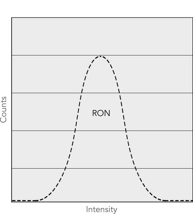 Readout noise histogram
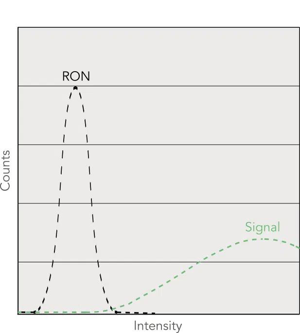
With low signal in regular CCDs, only a few photoelectrons are generated and so the signal will be of low intensity on the histogram. If this signal intensity is too low and falls in the same range as the readout noise, there is no way to distinguish between noise and signal, leading to inconclusive results.
 CCD acquisition histogram
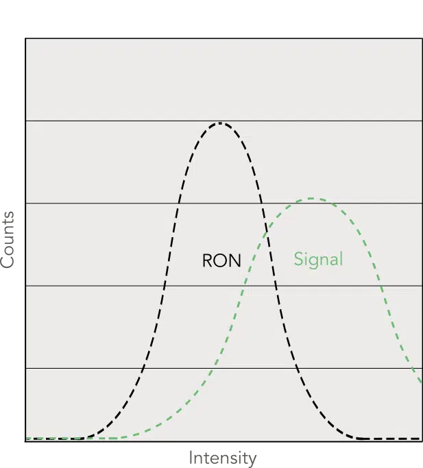
By using EM Gain, EMCCDs amplify the signal several orders of magnitude before digitization of the photoelectrons. This means even if the measured signal is very low, a large number of electrons will be read. As such, the readout noise will be distinct from the signal in the histogram. This is why readout noise is considered negligible in EMCCDs.
 EMCCD acquisition histogram
Without readout noise, smaller noise sources must be considered with EMCCDs. Dark current (i.e. thermal noise) occurs due to the thermal agitation of the sensor and increases linearly with exposure time (characterized in e/pixel/second). The sensor’s temperature is the only parameter that influences dark current.
As dark current is time-dependent and EMCCDs are deep cooled (<-50°C), it becomes negligible when using shorter exposures times; which is the norm in photon counting acquisitions. The final noise source is clock-induced charges (also known as spurious events), generated by the clock signals used to move charges on the EMCCD chip. This noise source is fixed per image (e/pixel/frame) and so becomes the dominant noise source in photon counting. Reducing clock-induced charges is critical to both linear and photon counting imaging.
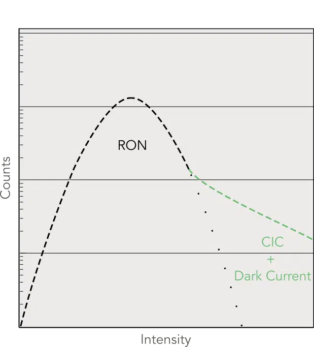
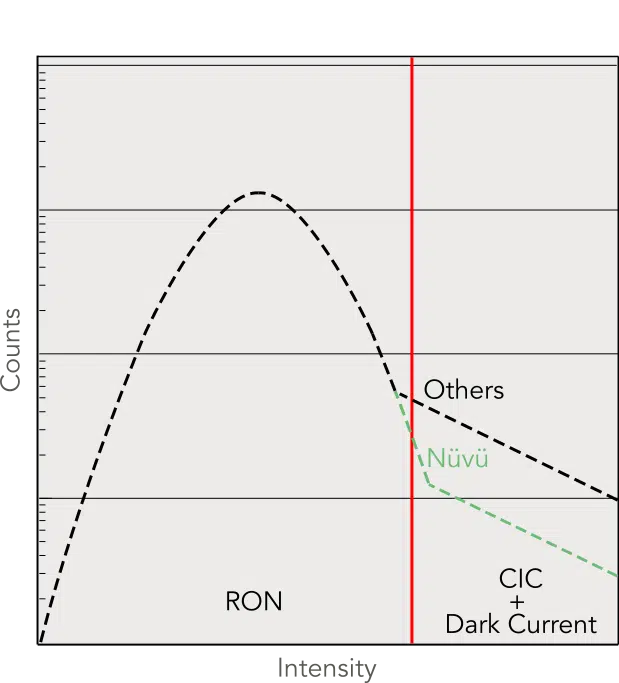
With EM Gain, the histogram of EMCCD dark frames shows a combination of the readout noise Gaussian and a tail created by both the clock-induced charges (CIC) and dark current. This histogram can be used to compare the performances of different EMCCD cameras and is at the base of photon counting thresholding.
 EMCCD dark frame histogram
With photon counting, instead of an image displaying intensity/pixel you obtain a binary image with 0 or 1 in each pixel (0 for no photon and 1 for a photon). This process is what allows to eliminate the excess noise factor, as the exact intensity value of each pixel is no longer important to the measurement; the photon counting image only measures whether a pixel was hit by a photon or not.
This technique is not only used in EMCCDs but also in e.g. avalanche diodes, X-Ray imaging. To achieve this binary image, an intensity threshold is set and if a pixel’s intensity is under the threshold no photon has hit the pixel whereas if the intensity is over the threshold, the pixel has been hit by a photon. This threshold can be clearly illustrated on a histogram.
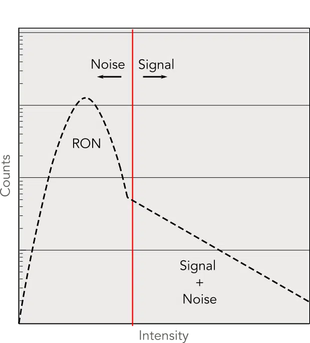 How thresholding applies to an EMCCD acquisition histogram.
Correctly establishing the threshold is crucial, as it must be low enough to capture a high number of photons but high enough to avoid registering too many noise events. A standard way to base the choice of a threshold is by using a measure of the standard deviation (σ) of the readout noise’s Gaussian curve. For EMCCDs, a universally recognized interval of confidence is achieved with a 5σ threshold. As such, there is only a 1 out of 3 million chance that readout noise on a pixel registers as a photon. Advanced users can select their own specific threshold according to their application and signal flux.
 Selecting an optimized threshold is crucial to image quality. A threshold too low compared to the readout noise standard deviation (σ) detects too much noise whereas a threshold too high cuts off too much signal.
Using high EM Gain is crucial for efficient photon counting as EM Gain increases the intensity of the signal, pushing the signal farther away from the readout noise Gaussian and allowing more photons to be detected above the threshold.
It could be inferred that using the highest EM Gain possible would be ideal in all cases but higher EM Gain also increases the clock-induced charges (CIC). Unlike readout noise, this noise source is generated on the detector and is multiplied along with signal photoelectrons. If the CIC gets too preeminent, the benefits of using higher EM Gain are cancelled.
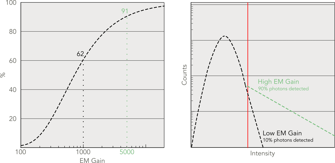 Left: Photon detection probability increases with higher EM Gain. Right: Image histogram showcasing the effect of higher EM Gain when using thresholding.
Most EMCCD camera manufacturers will cap their maximum EM Gain at ~1000, to prevent the user from acquiring images dominated by their higher CIC. However, this EM Gain is insufficient to use EMCCD photon counting efficiently and will offer minimal to no benefits compared to linear mode (LM) operation even though the ENF is eliminated. Although photon counting (PC) is a powerful acquisition technique, other manufacturers will rarely promote photon counting due to these stringent performance requirements.
 Impact of noise in a dark frame
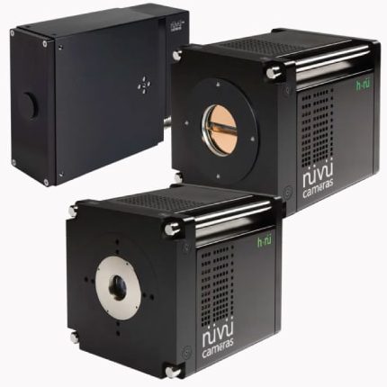
Thanks to Nüvü Camēras’ patented technology that significantly reduces CIC, our EMCCD detectors can operate at an EM Gain of up to 5000 while keeping CIC in check allowing unmatched photon counting performances. Nüvü’s photon counting has remained the choice of the most rigorous EMCCD users in demanding low light applications.
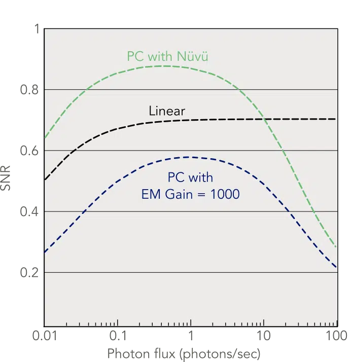 Signal to noise ratio (SNR) of EMCCD acquisition modes. The linear acquisitions use 1 image/sec and photon counting (PC) acquisitions use 10 images/sec.
Stacking photon counting images is very useful to produce a more comprehensive image with a dynamic range and encompassing your dataset. However, CIC are fixed per image (e/pixel/frame). Each frame added in a stack will also add its own CIC value. If an image with 50 levels is created, the image contains 50 times the amount of CIC found in a single image. This consideration makes it even more crucial to have the lowest CIC possible.
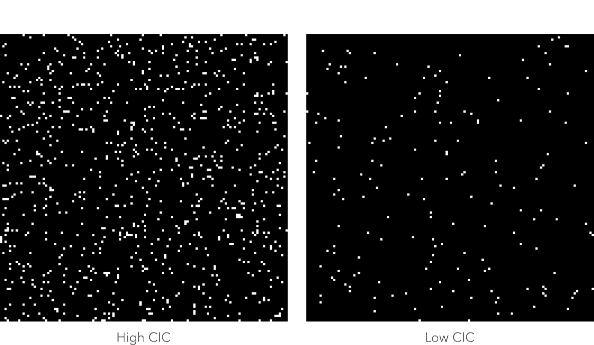 Image stacking with different CIC levels
Not all photon counting (PC) acquisitions are equal, as camera specifications play a key role in the final results. Even though thresholding eliminates the excess noise factor (ENF), if the camera’s performances are insufficient, photon counting will never actually lead to a gain in SNR; there will be too much noise and not enough signal above the threshold.
Most EMCCD detectors on the market are not appropriate for photon counting but Nüvü Camēras’ proprietary EMCCD electronics are designed for high-performance photon counting.
If you are interested in a more in-depth analysis of the mathematics & statistics supporting PC with EMCCD detectors as well as some additional data, there are several articles available for your consultation. Many more general questions are also answered in our EMCCD FAQ.