Astronomical imaging is always limited by the detection system signal-to-noise ratio (SNR). EMCCD cameras offer many advantages for low light applications, such as sub-electron read-out noise, and low dark current with appropriate cooling. High frame rate achieved with these devices is often employed for the enhancement of SNR by acquiring and stacking multiple short exposures instead of one long exposure. EMCCDs are also suitable for applications requiring very long exposures, even when only a few photons are detected per hour. During long exposure acquisitions with a conventional CCD, slower pixel rates are usually employed to reduce the read-out noise, which dominates the CCD noise budget. For EMCCD cameras, this approach may not result in the lowest possible total noise and the effect of increasing the total exposure time may not yield the highest possible SNR for a given total integration time. In this paper, we present and discuss the experimental results obtained with an EMCCD camera that has been optimized for taking long exposures (from several seconds to several hours) of low light-level targets. These results helped to ascertain an EMCCD camera best operating parameters for long exposure astronomical imaging.
Article publié dans SPIE Astronomical Telescopes + Instrumentation, 2014, Montréal, Quebec, Canada
Direct detection of exoplanets via coronagraphy is an increasingly important area of astronomical research. The advantages of a coronagraph operating at visible wavelengths include the possibility to measure key biomarkers O2, O3 and H2O as well as biologically important molecules CH4 and CO2 on early Earth analog.1 Additionally, an optical system optimized for visible spectral range observations would support the use of smaller telescopes rather than larger mid-IR telescopes to attain the required resolution. Better still, such system would operate at room temperature, thus eliminating the need for cryogenic cooling. Recently, several concepts for medium- or flagship-scale missions using coronagraphs have been investigated.2, 3 These studies have exposed the main technical difficulties of direct planet detection, namely the very high contrast between planets and their host stars as well as their small angular separation. Since it will be extremely challenging to reach the 10−9 contrast detection goal at 100 mas for wavelengths greater than 500 nm, photon-counting electron multiplying CCDs (EMCCDs) having high quantum efficiency (QE) in the visible and near-IR (0.4-1.1 µm) ranges with low dark current and read noise have been identified as a critical component of any exoplanet direct imaging mission.2, 4 Furthermore, it has been theoretically demonstrated4 that even in the ideal case of noise-free performance detector, integration times may extend from 1 second to over 100 hours. However, data acquisition with a conventional CCD generally calls for slower pixel rates to reduce the read-out noise, the dominating CCD noise source. For EMCCD cameras, data may not achieve the lowest noise from this procedure, and increasing integration time will not yield the highest SNR.
In our previous publications,5, 6 we have presented the many advantages of EMCCDs for low light applications: subelectron read-out noise, low dark current with appropriate cooling, and SNR enhancement by acquiring and stacking multiple exposures instead of one exposure due to the high frame rate achieved with these devices. In this paper, we report on a series of experiments designed to investigate the EMCCD potential for applications requiring very long exposures when only a few photons are detected per hour. The results obtained with integration times ranging from several seconds to several hours can be applied to optimize observation strategies for ground-based and spaceborne telescopes operating EMCCD low-light imaging cameras.
Measurements were performed at Nüvü Camēras with the EMN2 1k×1k EMCCD camera. The camera was the very first to use the third generation of CCCP controller (CCCPv3) and incorporates a grade-1 CCD201-20 EMCCD from e2v Technologies. The camera’s LN2 cooling system was tuned to stabilize the chip’s temperature between −85 and −115◦C.
2.1 Experimental set-up
The experimental set-up consisted of an Organic Light Emitting Diode (OLED) RGB display (4D systems µOLED-128- G2-REV3) which was employed as a photon source inserted into a light-tight tube attached to the EMN2’s front plate. Connected to the camera was a Thorlabs MVL7000 C-Mount lens looking directly at the display. A ND-6 filter (Thorlabs NE2R60B) was placed in front of the lens to attenuate the light emitted by the display, and the lens aperture was set to f/16. As the pixels of the display do not provide a 100% fill factor, the lens was slightly put out of focus to blur the display’s pixels and provide a more uniform illumination.
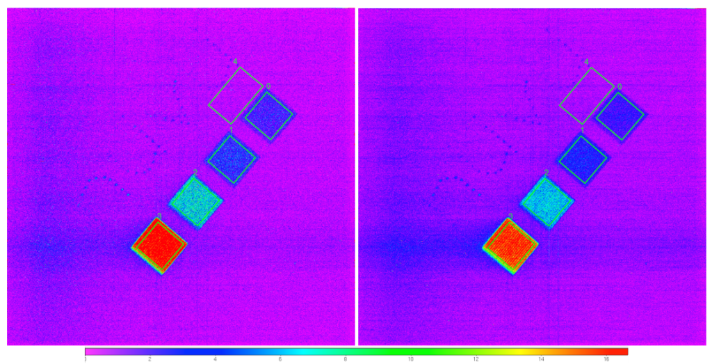
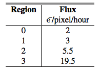
The OLED display was oriented at a 40 degree angle relative to a horizontal plane. Only the display’s green pixels were used, and the light output of each pixel was characterized by measuring the dependence of photon flux as a function of pixel’s current in order to achieve the desired number of photons emitted per hour. The OLED display produced images at the focal plane consisting of 4 squares with different luminance levels (marked as 0, 1, 2, and 3) and the nüvü letters on top of each square (in reversed order) as well as a blank region (region 4 ü thereafter) for dark measurements. The letters consists of dots composed of a single pixel of the OLED display, and each pixel have the same mean illumination as its corresponding square. The squares’ mean illumination is summarized in Table 1.
2.2 Data acquisition and processing
Data were collected at temperatures of −85◦C, −95◦C, and −105◦C. 6 different exposure times per frame were used: 10 , 30 s, 90 s, 300 s, 900 s, and 1800 s. For every temperature and exposure time combination, a total of 3 hours of integration has been achieved. 200 bias frames (0 s integration) were also taken for every parameters combination.
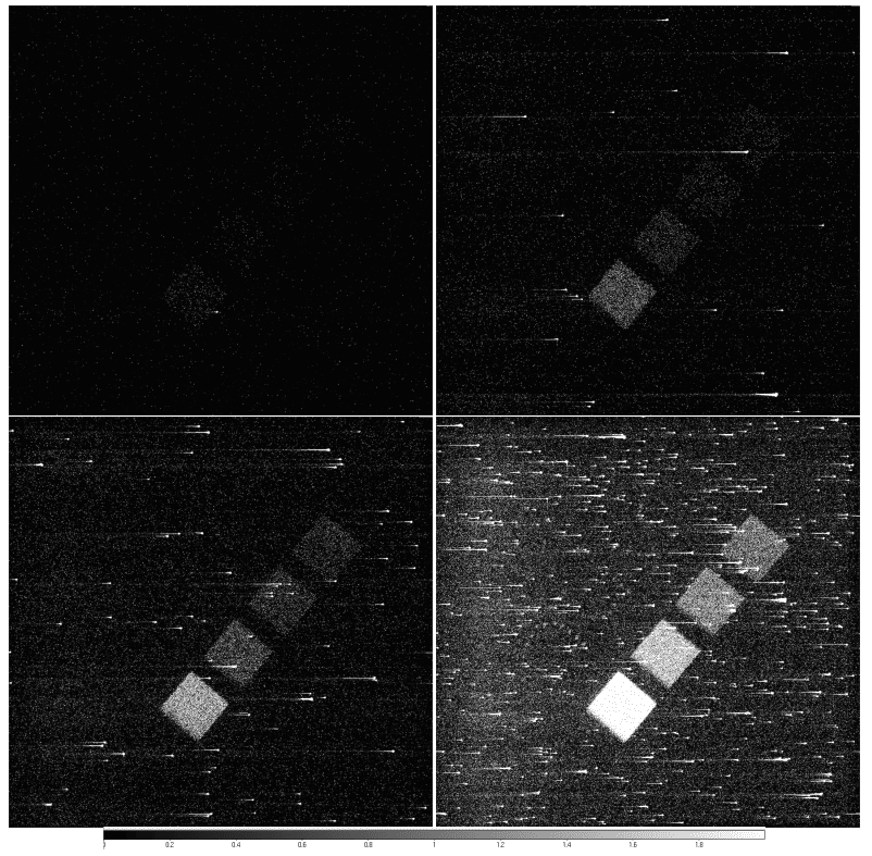
The EM gain of the camera was set to yield an EM gain over readout noise ratio of 40, leading to an effective read-out noise of 0.025 e¯ and a photon counting efficiency of >85%. The camera was operated in Inverted Mode Operation (IMO) at 10 MHz pixel rate to achieve the lowest level of total background signal (dark + CIC).6 Figure 2 presents a series images obtained at various exposure times.
Data were processed by first computing a master bias image with the acquired bias frames. It was then subtracted from the data frames to yield an 0 ADU reference image. Next, the stack of images was cleaned from cosmic rays with a sigmaclipping algorithm. Pixels flagged as being hit by a cosmic ray were replaced by the median value of the corresponding pixels in the other frames of the stack. The resulting data frames were subsequently divided by the EM gain, then summed to yield an image processed in analog mode (AM) where its values are expressed in electrons. The same data frames were also processed applying a threshold value equivalent to 5 times the readout noise (5×0.025 e¯), then summed to yield an image processed in photon counting mode (PC) where its values are also expressed in electrons. Figure 1 shows two resulting images of the same data being handled in AM and PC. This figure suggests that some of the background signal might consist of cosmic rays remnants, which explains the horizontal trails one can see in the unlit area of the images.
The processed data were analyzed to extract SNR and flux values from the signal regions outlined in Figure 1. The measured metrics were the total signal per pixel and the resulting SNR. From these, we computed an efficiency parameter to compare the data at various exposure times as well as processing methods (AM or PC).
3.1 Mean signal per pixel
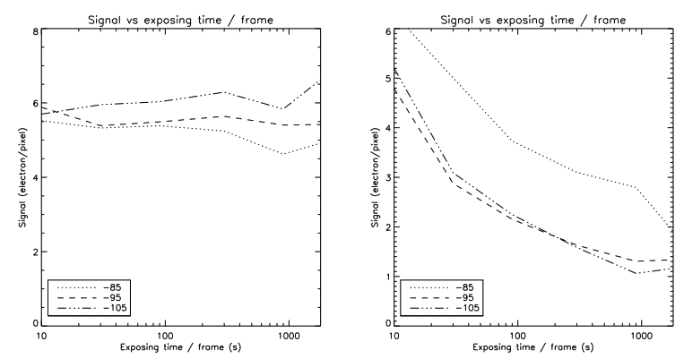
The mean signal per pixel was obtained by averaging the pixels’ values in the regions displayed in Figure 1, then subtracting the mean background signal. The left panel of Figure 3 presents the mean signal (background subtracted) measured in region 0 after 3 hours of integration as a function of the exposure time per frame. Data shows that the signal level is relatively stable, acquisition parameters notwithstanding. Even though such result was expected, it reveals the advantage of the EMCCD sub-electron read-out noise; the same total flux is measured in region 0 regardless of the flux per frame, which rises from 0.005 e¯/pixel/frame (10 s exposure time) to 1 e¯/pixel/frame (1800 s exposure time).
Figure 3 right panel presents the background signal for the same integration time. The declining background signal with increasing exposure time per frame is expected as less clock-induces charges (CIC) are being accumulated in the final image. For temperatures below −95◦C, the background signal is less than 1 electron/pixel/hour for exposure of more than 30 seconds.
One striking evidence of Figure 3 is the similarity between the background signal for temperatures of −105◦C and −95◦C. We supposed that cosmic rays residues might be a non-negligible background component.
As flux is independent of the operating temperature and the background signal is similar at −95◦C and −105◦C, we chose to use the −95◦C data set results for the following analysis.
3.2 SNR
The regions of interest’s SNRs are computed using the following equation:
SNR = S/σ , (1)
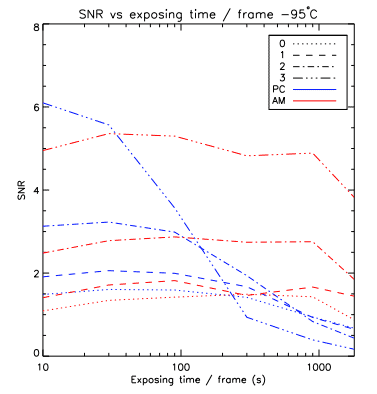
where S represents the mean signal (background subtracted), and σ is the standard deviation for the same region. Since all regions exhibit a diagonal pattern due to the OLED display fill factor, σ was calculated by processing the data for every acquisition parameters (temperature and exposure time) into two halves. The first half was subtracted from the second one and the standard deviation of the resulting image was determined for every region of interest. This operation increased σ by a factor of √ 2, while the use of only half of the data set will decrease the shot noise by a factor of √ 2. Hence, the computation of the standard deviation of the subtracted images directly provides σ. The corresponding SNRs are shown in Figure 4.
Figure 4 curves reveal the quick decrease of the SNR in PC with growing flux intensities because of the PC pixels saturation. The AM-processed data’s SNR remains relatively flat despite the change in exposure time. This point will be discussed later when comparing the efficiency parameters. However, all SNRs decrease for very long exposure time per frame, even in AM. One possible explanation is the improper removal of cosmic rays for these data sets. The very few images available (6 images for 1800 s) makes it hard for the sigma-clipping algorithm to distinguish between the tail left by a cosmic ray (see Figure 2) and the actual signal. These remnants artificially increase the variance, hence the observed decrease of the SNR.
3.3 Efficiency comparison
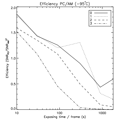
The efficiency is expressed as the square of the SNR ratio:
η = SNRb/SNRa 2 , (2)
η is the ratio of the total integration required to reach any given SNR when going from the acquisition parameters of a to the acquisition parameters of b. In the following analysis, the comparison point a is set as the 10 s of exposure per frame SNR data.
Figure 5 demonstrates the advantage of handling data in PC rather than analog mode for the faintest fluxes. At low flux, PC data handling provides a 30–50% efficiency gain for exposure times of ≤90 s. For higher fluxes and/or longer exposure times per frame, the advantage of PC over AM vanishes as PC pixels begin to saturate. It must be emphasized that both PC and AM processing were performed on the same data set, a decision being made after data acquisition. Hence, data handling can be adjusted as a function of the incoming flux to benefit from the best of the processing methods.
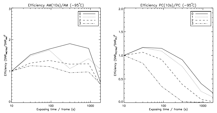
Figure 6 shows the efficiency comparison for the AM (left panel) and PC (right panel) processing. SNR peaks at 300 s per frame in AM while achieving its highest value in PC between 30 and 90 s (for the faintest region). For the brightest regions, in AM, the efficiency remains about the same exposure ≥30 s. These regions are dominated by the signal’s shot noise rather than background signal, thus the lack of efficiency increase with increasing exposures. As depicted in the previous section, η decreases for the very long exposure time per frame. Theoretically, there is no reason for such decline, except for the improper removal of cosmic rays.
One stunning conclusion one can draw from Figure 6 is the very little benefits brought by exposures greater than 30–90 s per frame, even for the faintest fluxes. In fact, there are disadvantages:
• As exposure time increases, pixels saturate at a lower flux, which will decrease the dynamic range;
• Cosmic rays become harder to filter out as there are less images to provide good statistics;
• The flux range within which PC processing has an advantage over AM is smaller, forcing the user to process data in AM and be impacted by the excess noise factor (ENF).
In this paper, we have demonstrated the distinct advantages of EMCCD imaging for astronomical applications requiring long exposures. By eliminating readout noise, the EMCCD prevents weak signals from being wiped out by the readout process, and provides dark-noise limited images in a matter of seconds rather than hours. Therefore, the integration time for a single frame can be significantly reduced without losing information; by comparison, a conventional CCD with comparable quantum efficiency will have to increase its total exposure time to obtain an adequate SNR in a shot noise limited regime. In order to realize the highest SNR, photon-counting processing is mandatory as it gets rid of the EMCCD’s inherent ENF. In this scheme, using several short exposures (≤100 s) for several hours total integration time provides better dynamic range. Moreover, the number of images gathered eases cosmic-ray filtering greatly, an important aspect for space applications.
Furthermore, results show that there is little impact on the SNR while resorting to exposures much shorter than 100 s. Figure 6 made clear that even for 10 s exposures, the impact on the total integration time required to reach the same SNR is about 20–30% for flux as low as 2 photons/pixel/hour, whilst this kind of acquisition will greatly increase the dynamic range of the data. As an added benefit, shorter exposures could relax the required pointing accuracy of a spacecraft as its stability would only need to be controlled on a few tens of seconds timescale rather than several minutes.
At last, it must be noted that all of our data were collected in inverted mode operation (IMO), which produces the lowest dark current6 at the price of an increased CIC level.7 The precise control of clocking parameters achieved with Nüvü Camēras’ version 3 controller allows to minimize the CIC to negligible levels even in IMO mode resulting in highest possible SNR that is the key to successful data acquisition with an EMCCD low-light imager operating with long integration times.
REFERENCES
[1] Kuchner, M. J. and Spergel, D. N., “Terrestrial Planet Finding with a Visible Light Coronagraph,” in [Scientific Frontiers in Research on Extrasolar Planets], Deming, D. and Seager, S., eds., Astronomical Society of the Pacific Conference Series 294, 603–610 (2003).
[2] Levine, M. et al., “Overview of Technologies for Direct Optical Imaging of Exoplanets,” in [astro2010: The Astronomy and Astrophysics Decadal Survey], Astronomy 2010, 37 (2009).
[3] Lyon, R. G., Clampin, M., Melnick, G., Tolls, V., Woodruff, R., and Vasudevan, G., “Extrasolar Planetary Imaging Coronagraph (EPIC): visible nulling cornagraph testbed results,” in [Society of Photo-Optical Instrumentation Engineers (SPIE) Conference Series], Society of Photo-Optical Instrumentation Engineers (SPIE) Conference Series 7010 (Aug. 2008).
[4] Shaklan, S., Levine, M., Foote, M., Rodgers, M., Underhill, M., Marchen, L., and Klein, D., “The afta coronagraph instrument,” (2013).
[5] Daigle, O., Quirion, P.-O., and Lessard, S., “The darkest EMCCD ever,” in [Society of Photo-Optical Instrumentation Engineers (SPIE) Conference Series], Society of Photo-Optical Instrumentation Engineers (SPIE) Conference Series 7742 (July 2010).
[6] Daigle, O., Djazovski, O., Laurin, D., Doyon, R., and Artigau, E., “Characterization results of EMCCDs for extreme ´ low-light imaging,” in [Society of Photo-Optical Instrumentation Engineers (SPIE) Conference Series], Society of Photo-Optical Instrumentation Engineers (SPIE) Conference Series 8453 (July 2012).
[7] “Low-light technical note 4 dark signal and clock-induced charge in l3vision ccd sensors,” tech. rep., E2V Technologies, http://www.e2v.com/shared/content/resources/File/documents/ imaging-space-and-scientific-sensors/Papers/low_light_tn4.pdf (June 2004).