


Abstract
The Gaia satellite recently released parallax measurements for ∼260,000 high-confidence white dwarf candidates, allowing for precise measurements of their physical parameters. By combining these parallaxes with Pan-STARRS and u-band photometry, we measured the effective temperature and stellar mass for all white dwarfs in the Northern Hemisphere within 100 pc of the Sun, and identified a sample of ZZ Ceti white dwarf candidates within the so-called instability strip. We acquired high-speed photometric observations for 90 candidates using the PESTO camera attached to the 1.6 m telescope at the Mont-Mégantic Observatory. We report the discovery of 38 new ZZ Ceti stars, including two very rare ultramassive pulsators. We also identified five possibly variable stars within the strip, in addition to 47 objects that do not appear to show any photometric variability. However, several of those could be variable with an amplitude below our detection threshold, or could be located outside the instability strip due to errors in their photometric parameters. In the light of our results, we explore the trends of the dominant period and amplitude in the M– plane, and briefly discuss the question of the purity of the ZZ Ceti instability strip (i.e., a region devoid of non-variable stars).
Export citation and abstract BibTeX RIS
1. Introduction
White dwarf stars represent the end product of 97% of the stars in the Galaxy. Their cores no longer produce energy through nuclear fusion, and so they slowly cool down over the span of billions of years, allowing us to interpret their temperature sequence as an evolutionary track. Most white dwarfs go through an instability stage at some point in their lives, depending on the chemical composition of their outer stellar envelope, during which they exhibit nonradial g-mode pulsations. For instance, once DA (hydrogen-line) white dwarfs reach an effective temperature between  K and ∼10,200 K (for a surface gravity of
  = 8, Gianninas et al. 2014), their internal conditions become prone to such pulsations, manifesting themselves as periodic variations in the luminosity of the star, with periods typically ranging from 100 s (Voss et al. 2006) to 2000 s (Green et al. 2015), and relative amplitudes from 0.1% to 40% (Mukadam et al. 2004).
One of the main interests surrounding the region in the  –
– plane containing the variable DAs, namely the ZZ Ceti instability strip, is to determine whether it is pure or not. A pure strip, devoid of any photometrically constant DA white dwarfs, would suggest that ZZ Ceti stars represent an evolutionary phase through which most, if not all, hydrogen-atmosphere white dwarfs are expected to cool. We could then use asteroseismology as a tool to study the internal structure not only of ZZ Ceti stars, but also of the population of DA white dwarfs as a whole (Giammichele et al. 2017). On the other hand, an impure strip containing a mix of variable and non-variable DA stars would imply a missing parameter in our evolutionary models (Fontaine & Brassard 2008). The purity of the instability strip has a long history of swinging back and forth between these two possibilities. On one hand, there are studies such as that of Gianninas et al. (2014), who restricted their sample to only the brightest ZZ Ceti stars with high signal-to-noise spectra, and whose results point toward a pure instability strip. But there are also many studies claiming the strip to be populated with both variable and non-variable stars (see, for example, Mukadam et al. 2005). In most of those cases, the photometrically constant stars were either found to be variable when using better instruments (Castanheira et al. 2007) or proven to be located outside the strip by measuring their parameters with higher-quality data (Gianninas et al. 2005). Even though it is an uphill battle, the consensus seems to be slowly heading toward a pure strip.
Over the years, there have been many efforts to define the spectroscopic ZZ Ceti instability strip both empirically and theoretically. The theoretical determination of the strip edges is still a work in progress, because it depends strongly on the physical assumptions made in these studies, especially when it comes to the efficiency of convective energy transport (see Fontaine & Brassard 2008; Althaus et al. 2010, and Córsico et al. 2019 for excellent reviews on the subject). Furthermore, the assumptions behind the theoretical edges are often based on their empirical locations, which are themselves dependent on a variety of factors, such as the signal-to-noise ratio of the spectra (Gianninas et al. 2005). Building a large, homogeneous sample of photometrically variable and constant stars inside and near the instability strip is the first step toward a robust determination of the empirical edges. Bergeron et al. (1995) began this venture by collecting time-averaged optical spectra to measure the  and
and  values of known ZZ Ceti stars, allowing them to select new ZZ Ceti candidates with high confidence. Since then, this so-called spectroscopic technique has been used repeatedly to identify new ZZ Ceti stars, with perhaps the most impressive of these studies being that of Mukadam et al. (2004), who reported in a single paper the discovery of 35 new ZZ Ceti stars in the Sloan Digital Sky Survey (SDSS) and the Hamburg Quasar Survey. In parallel, the same approach has been used to constrain the exact location of the ZZ Ceti instability strip by also studying non-variable DA white dwarfs around the strip (see, e.g., Gianninas et al. 2005). By far, the spectroscopic technique has been the go-to method to identify new candidates, being one of the main contributors of the ∼200 new ZZ Ceti stars found in the last 20 years or so (Bognar & Sodor 2016).
Unfortunately, the determination of the exact location of the empirical ZZ Ceti instability strip has been hampered by the use of different model atmospheres in these spectroscopic investigations, which differ in terms of the Stark broadening theory for the hydrogen lines, as well as different assumptions about the convective efficiency. More importantly, Tremblay et al. (2011) demonstrated that the mixing-length theory used to describe the convective energy transport in previous model atmosphere calculations was responsible for the apparent increase in spectroscopic  values below
  K, a problem that could be solved by relying on realistic 3D hydrodynamical model atmospheres (Tremblay et al. 2013). Given this confusing situation, we decided to revisit this problem more quantitatively in a homogeneous fashion.
Our starting point is the study of Green et al. (2015), who presented new high-speed photometric observations of ZZ Ceti white dwarf candidates drawn from the spectroscopic survey of bright DA stars in the Villanova White Dwarf Catalog (McCook & Sion 1999) by Gianninas et al. (2011), and from the spectroscopic survey of white dwarfs within 40 pc of the Sun by Limoges et al. (2015). Figure 2 of Green et al. summarizes the distribution of  as a function of
  for all ZZ Ceti and photometrically constant white dwarfs in their sample, providing us with an empirical instability strip based on the largest (and mostly) homogeneous sample yet. However, their spectroscopic solutions, obtained from model atmospheres based on the ML2/α = 0.7 version of the mixing-length theory, were not corrected for hydrodynamical 3D effects. Here we first apply the 3D corrections from Tremblay et al. (2013) to the spectroscopic
  and
and  values, and then convert the
  values into stellar masses (M) using evolutionary models described in Section 2. The resulting distribution of white dwarfs in the M–
 plane is displayed in Figure 1. We use these results to derive improved empirical boundaries for the ZZ Ceti instability strip, also reproduced in Figure 1, which will serve as a reference in our discussion below. The 3D hydrodynamical corrections can be neglected in the context of photometric analyses, as discussed by Tremblay et al. (2013), who showed that 1D or 3D-corrected models yield similar results for DA white dwarfs in the temperature range 7000–14,000 K (see their Figure 16).
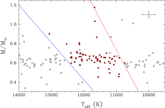
Figure 1. Distribution of the ZZ Ceti stars (red) and photometrically constant white dwarfs (white) from Green et al. (2015) in the M– plane. Here the spectroscopic parameters have been corrected for hydrodynamical 3D effects. The cross in the upper right corner represents the average uncertainties in both parameters. The empirical ZZ Ceti instability strip is indicated by the blue (hot edge) and red (cool edge) lines.
Download figure:
Standard image High-resolution imageWith the second Gaia data release, trigonometric parallaxes have become available for an unprecedented number of white dwarf stars, opening a whole new window of opportunity to identify new ZZ Ceti stars. Indeed, distances derived from such parallaxes are an essential ingredient for precise measurements of their physical parameters using the so-called photometric approach. In this paper, we make use of the Panoramic Survey Telescope and Rapid Response System (Pan-STARRS) photometry for the first time in the context of identifying new ZZ Ceti stars and constraining the empirical edges of the photometric ZZ Ceti instability strip. By combining Gaia astrometric data with this nearly all-sky photometric survey, at least in the Northern Hemisphere, we obtain one of the largest photometric samples of ZZ Ceti candidates yet. This combination of parallax and photometric data has been thoroughly investigated by Bergeron et al. (2019), who showed that physical parameters—namely  and M—derived from spectroscopy and photometry reveal systematic offsets (see their Figure 4). We thus expect the empirical ZZ Ceti instability strip obtained from our photometric analysis to exhibit similar offsets with respect to spectroscopic determinations.
Our selection of ZZ Ceti candidates is first discussed in Section 2, while the high-speed photometric follow-up program for our selected ZZ Ceti candidates, as well as the data reduction procedure, are described in Section 3. Our results, including the discovery of 38 (and possibly 43) new ZZ Ceti stars and the discussion of the empirical photometric instability strip, are presented in Section 4. Our conclusions follow in Section 5.
2. Candidate Selection
Our initial sample consists of all objects from the Gaia Data Release 2 (Gaia Collaboration et al. 2016, 2018b) within 100 pc of the Sun and parallax measurements more precise than 10%. This distance limit was chosen so that interstellar reddening could be neglected in our photometric analysis described below (Harris et al. 2006). To define our white dwarf candidate sample, we apply the selection criteria described in Section 2.1 of Gaia Collaboration et al. (2018a) excluding the limits on flux_over_error for G, GBP, and GRP magnitudes. More specifically, we select objects with an absolute Gaia magnitude  and color indices
  . Figure 2 shows the Gaia color–magnitude diagram for the 12,857 objects contained in this initial sample. We note that this selection of white dwarf candidates excludes the extremely low-mass (ELM) white dwarf pulsators (Bell et al. 2017), because they are located significantly above the white dwarf sequence in the Gaia color–magnitude diagram (Gaia Collaboration et al. 2019). However, all of the currently known ELM pulsators have distances of the order of kiloparsecs (Brown et al. 2011), and their number within 100 pc is expected to be extremely small (Kawka et al. 2020).
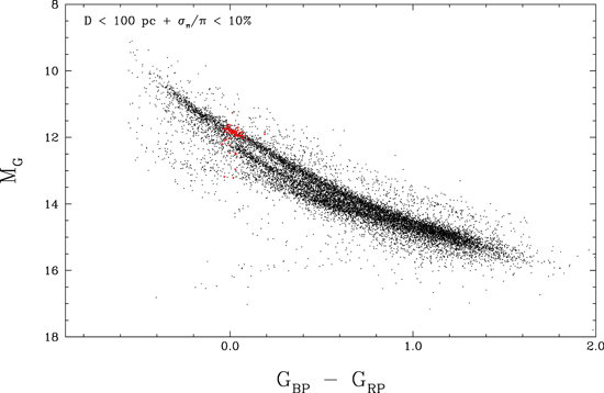
Figure 2. Color–magnitude diagram for Gaia white dwarfs and white dwarf candidates within 100 pc of the Sun with parallax measurements more precise than 10%. Our search for pulsating ZZ Ceti pulsators is based on this parallax- and color-selected sample containing 12,857 objects. Previously known ZZ Ceti stars are shown in red.
Download figure:
Standard image High-resolution imageWe then cross-match this initial sample with the Pan-STARRS Data Release 1 catalog (Chambers et al. 2016) using the following algorithm.1 For each Gaia object, a first query is made at the Gaia coordinates in a circle of 5'' radius, and if only one object is found and has good quality flags, it is chosen as the cross-match. If no objects are found, we expand the radius of the search query to 20''. If multiple Pan-STARRS objects are found within this search radius, the Gaia object is looked up on the SIMBAD Astronomical Database (Wenger et al. 2000) for SDSS ugriz magnitudes (York et al. 2000). Since SDSS and Pan-STARRS griz filters are comparable, we use available SDSS photometry to select the Pan-STARRS object with the closest matching photometry, allowing a difference of up to 0.3 mag per filter. In the case where no Pan-STARRS objects meet this criteria, the cross-match fails. If no SDSS photometry is available, we use instead the G − r relationship described in Evans et al. (2018) to estimate an SDSS r magnitude and select the object with the closest Pan-STARRS r magnitude, up to a difference of 0.7 mag.
With the Gaia parallaxes and Pan-STARRS grizy photometry in hand, every object in our initial sample is fitted using the photometric technique described at length in Bergeron et al. (1997), together with the pure hydrogen2
and pure helium model atmospheres discussed in Bergeron et al. (2019) and references therein. As mentioned above, given the distance limit of our sample, interstellar reddening is neglected altogether. The fitted parameters are the effective temperature,  , and the solid angle, π(R/D)2, where R is the radius of the star and D its distance from Earth, derived from the trigonometric parallax measurement. The fitted stellar radii can be converted into surface gravity (
 ) and stellar mass (M) using evolutionary models3
similar to those described in Fontaine et al. (2001) with (50/50) C/O-core compositions,
) and stellar mass (M) using evolutionary models3
similar to those described in Fontaine et al. (2001) with (50/50) C/O-core compositions,  , and q(H) = 10−4 or 10−10 for the pure hydrogen and pure helium solutions, respectively. As discussed in the Introduction, 3D hydrodynamical corrections can be neglected in the context of photometric analyses (Tremblay et al. 2013).
In Figure 3, we show a typical fit for one object in our sample using Pan-STARRS grizy photometry and the Gaia parallax measurement. As can be seen from this result, hydrogen- and helium-atmosphere white dwarfs can be difficult to distinguish based on Pan-STARRS grizy photometry alone, because their average flux distributions at 0.4–1.0 μm tends to be quite similar. To overcome this problem, we supplement our set of grizy photometry with u-band photometry, if available, taken from the SDSS or from the ongoing Canada–France Imaging Survey (CFIS) described in Ibata et al. (2017). The wavelength coverage of the u bandpass includes the Balmer jump, which is a very distinctive feature between hydrogen- and helium-atmosphere white dwarfs. Indeed, hydrogen-atmosphere white dwarfs have a significant drop in u-band flux, whereas their helium-atmosphere counterparts have a more continuous flux distribution. The u magnitude is not included in the fitting procedure but it is used instead in our analysis (see below) to discriminate between the pure hydrogen and pure helium solutions, as illustrated in Figure 3, where the drop in the u-flux caused by the Balmer jump is accurately reproduced by the pure hydrogen model.
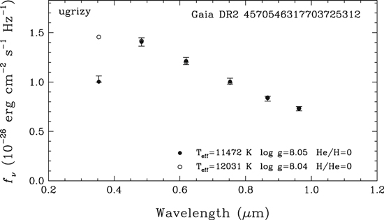
Figure 3. Sample photometric fit to a ZZ Ceti white dwarf candidate using Pan-STARRS grizy and CFIS-u photometry (error bars), combined with the Gaia parallax measurement. Filled circles correspond to our best fit under the assumption of a pure hydrogen atmospheric composition, while the open circles assume a pure helium atmosphere. Note that the CFIS-u data point is not used in these fits and serves only to discriminate between the pure hydrogen and pure helium solutions (see text); the results clearly indicate that this object is a hydrogen-atmosphere white dwarf.
Download figure:
Standard image High-resolution imageThe photometric fits are also useful to identify non-white dwarf objects when the measured parameters are unrealistic, in particular the stellar radius. However, it is also possible to obtain a bad fit if our photometric cross-match is erroneous, in which case we may miss white dwarf candidates in our initial sample. These two scenarios affected less than 1% of the objects with a Pan-STARRS cross-match.
The stellar masses for all objects in our sample are displayed in Figure 4 as a function of effective temperature; here a pure hydrogen atmospheric composition is assumed for all objects. The upper panel shows the full M– distribution of our sample. As discussed in detail by Bergeron et al. (2019), the large masses observed below
  K correspond to helium-atmosphere white dwarfs containing small traces of hydrogen (or carbon and other heavy elements), whose masses are overestimated when analyzed with pure hydrogen or even pure helium model atmospheres.

Figure 4. Top: distribution of the objects in our sample in the M– plane, measured using the photometric technique assuming pure hydrogen atmospheres. The spectroscopic (dashed lines) and photometric (solid lines) empirical ZZ Ceti instability strips are indicated by the blue (hot edge) and red (cool edge) lines. Bottom: same as the top panel, but zoomed in on the instability strip; the cross in the lower left corner represents the average uncertainties in both parameters. Known ZZ Ceti (magenta), DA (yellow), and non-DA (cyan) white dwarfs are also identified.
Download figure:
Standard image High-resolution imageOf more interest in the present context is the range of effective temperature where ZZ Ceti white dwarfs are expected, displayed in the bottom panel of Figure 4. Also reproduced in both panels (dashed lines) is the location of the ZZ Ceti instability strip determined empirically by Green et al. (2015, see Figure 1). In principle, this instability strip could be used to select our ZZ Ceti candidates for follow-up high-speed photometry. However, as demonstrated by Bergeron et al. (2019), photometric temperatures obtained from Pan-STARRS grizy photometry are significantly lower than spectroscopic temperatures. We reproduce in Figure 5 the results from Bergeron et al. (their Figure 4) but only for the range of temperature of interest. We can see that the temperature offset varies slightly as a function of  , but that it is otherwise well defined on average. We thus use the results displayed in Figure 5 to apply a temperature correction to the spectroscopic instability strip determined by Green et al. (2015) to estimate the photometric boundaries of the strip, as indicated by solid lines in Figure 4. This is the region of the M–
 plane that will be used to define our sample of ZZ Ceti candidates.
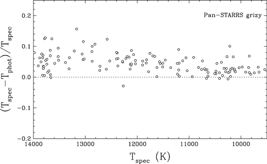
Figure 5. Differences between spectroscopic and photometric effective temperatures as a function of  for DA stars in the region of interest, drawn from the sample of Gianninas et al. (2011), using photometric fits to the Pan-STARRS grizy data. The dotted line indicates equal temperatures.
Download figure:
Standard image High-resolution imageAnother concern is the omission of the u-band photometry to estimate our effective temperatures. Indeed, Bergeron et al. (2019, see their Figures 4 and 7) demonstrated that a much better agreement between photometric and spectroscopic temperatures could be achieved if the SDSS u magnitude was combined with the Pan-STARRS grizy photometry. To explore this effect, we compare in Figure 6 the difference between effective temperatures obtained by fitting Pan-STARRS grizy photometry alone and the values obtained by also including the u magnitude (SDSS or CFIS) for objects within the ZZ Ceti region. In this figure, different colors are used to distinguish hydrogen- and helium-atmosphere candidates. Our results indicate that for hydrogen-atmosphere white dwarfs in the range of temperature of interest for our survey, the use of additional u-band photometry has little effect on the estimated photometric temperatures, with no systematic offset observed, and a standard deviation of only 1.2%.
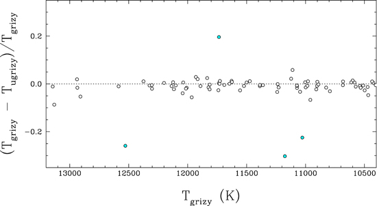
Figure 6. Differences between photometric temperatures measured using only Pan-STARRS photometry (Tgrizy) and those obtained by also including SDSS or CFIS u-band photometry (Tugrizy) for objects within the ZZ Ceti region. The dotted line indicates equal temperatures. White and cyan symbols correspond, respectively, to hydrogen- and helium-atmosphere candidates.
Download figure:
Standard image High-resolution imageThe photometric instability strip displayed in the bottom panel of Figure 4 can now be used to define a region that contains 286 objects. From this list, we remove all known ZZ Ceti pulsators taken from the compilation of Córsico et al. (2019) as well as recent discoveries (Romero et al. 2019); these are indicated by magenta symbols in the bottom panel of Figure 4. Incidentally, the locations of these known variables are perfectly well bracketed by our empirical photometric instability strip, giving us confidence in our overall procedure.
Known helium-atmosphere white dwarfs—cyan symbols in the bottom panel of Figure 4—are also removed by comparing our list against the MWDD and SIMBAD. Candidates with u magnitudes indicating a helium-rich atmosphere, through our fitting procedure mentioned above, are also removed. While in principle this procedure could be used to exclude all the remaining unidentified helium-atmosphere candidates, u magnitudes are only available for less than half of the objects in our sample. Among the remaining candidates with available u magnitudes, about 26% were removed through the fitting procedure, and so we expect a similar proportion of helium-atmosphere white dwarfs to contaminate our list of ZZ Ceti candidates with neither a u-band measurement nor known spectral information. The SDSS is the largest source of u magnitudes in our sample, but unfortunately it does not cover as much sky as the Gaia survey. The CFIS survey, currently under way,4 should eventually provide u-band photometry for additional targets in our sample. While its sky coverage mostly overlaps with SDSS, the photometry will be approximately 3 mag deeper than SDSS for a given measurement uncertainty (Ibata et al. 2017). The CFIS u magnitudes have been consistent with our model predictions so far, as displayed in Figure 3.
Finally, objects in the Southern Hemisphere (δ < −10°) are also excluded from our target list due to the location of the Mont-Mégantic Observatory, where our high-speed photometric observations were secured. At the end, our final sample contains 173 ZZ Ceti candidates, out of which 80 are confirmed to be hydrogen-rich through u-band photometry. This list of candidates, in addition to 18 objects just outside the blue edge, is presented in Table 1 and is available as supplementary material.
Table 1. Observational Data for the List of ZZ Ceti Candidates
| Column Number | Units | Explanation |
|---|---|---|
| 1 | ⋯ | Gaia DR2 identifier |
| 2 | deg | R.A. in decimal degrees (J2015.5) |
| 3 | deg | Decl. in decimal degrees (J2015.5) |
| 4, 5 | mas | Parallax and error |
| 6, 7 | mas yr−1 | Proper motion in R.A. |
| 8, 9 | mas yr−1 | Proper motion in decl. |
| 10 | mag | Gaia DR2 mean G band magnitude |
| 11 | mag | Gaia DR2 blue passband magnitude |
| 12 | mag | Gaia DR2 red passband magnitude |
| 13, 14 | mag | Pan-STARRS g band magnitude |
| 15, 16 | mag | Pan-STARRS r band magnitude |
| 17, 18 | mag | Pan-STARRS i band magnitude |
| 19, 20 | mag | Pan-STARRS z band magnitude |
| 21, 22 | mag | Pan-STARRS y band magnitude |
| 23, 24 | mag | Canada–France Imaging Survey u-band magnitude |
| 25, 26 | mag | SDSS u-band magnitude |
Only a portion of this table is shown here to demonstrate its form and content. A machine-readable version of the full table is available.
Download table as: DataTypeset image
3. Data Acquisition and Reduction
We obtained time series photometry using the PESTO camera on the 1.6 m telescope at the Mont-Mégantic Observatory (Québec). Our survey spanned over 68 nights from 2018 July to 2020 August, using a mix of classical and queue observing. We used a 10 s exposure time for most observations, occasionally increasing to 30 s for fainter objects. We initially used a g' filter5
but eventually switched to using no filter to maximize the target flux and signal-to-noise ratio. For an exposure time of 10 s, we achieved a typical photometric precision of 2.6% for objects with Gaia magnitudes 15.5 < G < 16.5, and 4.7% for objects with  . Our journal of observations is presented in Table 2.
Table 2. Journal of Observations
| Date at Start | Gaia Source ID | Duration | No. of | Exposure | Filter |
|---|---|---|---|---|---|
| (UT) | (hr) | Images | (s) | ||
| 2020-08-13 04:01:06 | 2863526233218817024 | 1.5 | 361 | 15 | None |
| 2020-08-13 05:40:04 | 2779284538516313600 | 1.3 | 451 | 10 | None |
| 2020-08-13 07:01:05 | 2789405753503977472 | 1.5 | 361 | 15 | None |
| 2020-08-11 02:35:41 | 2867203584218146944 | 1.0 | 241 | 15 | None |
| 2020-08-8 02:11:13 | 4503347770490390016 | 1.5 | 361 | 15 | None |
| 2020-08-8 03:53:26 | 1815614965310875520 | 1.5 | 361 | 15 | None |
| 2020-08-8 05:28:25 | 1930609656643838080 | 1.5 | 361 | 15 | None |
| 2020-08-7 03:21:24 | 4298401105174809984 | 1.9 | 451 | 15 | None |
| 2020-08-7 05:08:55 | 1980205739970324224 | 1.7 | 408 | 15 | None |
| 2020-08-7 06:53:00 | 1993426577008368640 | 1.6 | 381 | 15 | None |
| 2020-07-29 03:56:58 | 4539136259802013952 | 1.3 | 451 | 10 | None |
| 2020-07-22 03:15:46 | 2292229788249205760 | 1.6 | 559 | 10 | None |
| 2020-07-16 02:56:53 | 2092086476924423808 | 2.2 | 522 | 15 | None |
| 2020-07-16 05:22:28 | 2063435712171048704 | 1.3 | 451 | 10 | None |
| 2020-07-10 03:38:09 | 1353302001211658368 | 1.6 | 381 | 15 | None |
| 2020-07-7 05:59:56 | 2127591833389528064 | 2.0 | 484 | 15 | None |
| 2020-06-20 06:39:37 | 2163226700308494080 | 1.3 | 313 | 15 | None |
| 2020-06-19 04:49:00 | 1968901145520461568 | 1.6 | 376 | 15 | None |
| 2020-06-19 03:22:53 | 1411867767238390912 | 1.3 | 451 | 10 | None |
| 2020-06-19 06:50:59 | 2220815923910913920 | 1.3 | 451 | 10 | None |
| 2020-06-18 02:34:25 | 1353355434900703616 | 1.3 | 451 | 10 | None |
| 2020-06-17 03:23:41 | 575585919005741184 | 2.0 | 241 | 30 | None |
| 2020-06-17 05:41:34 | 1845487489350432128 | 2.0 | 241 | 30 | None |
| 2020-06-16 06:36:04 | 1344618951728016512 | 1.3 | 451 | 10 | None |
| 2020-06-16 01:51:35 | 575585919005741184 | 2.3 | 271 | 30 | None |
| 2020-06-12 01:47:26 | 2114985726416563072 | 2.3 | 278 | 30 | None |
| 2020-06-6 01:33:41 | 1411867767238390912 | 1.6 | 566 | 10 | None |
| 2020-03-15 23:43:00 | 3169486960220617088 | 1.9 | 700 | 10 | None |
| 2020-03-16 08:10:55 | 1317275544951049472 | 2.0 | 717 | 10 | None |
| 2020-02-15 06:48:28 | 3626525219143701120 | 2.0 | 721 | 10 | None |
| 2020-01-31 07:10:47 | 642549544391197440 | 2.0 | 721 | 10 | None |
| 2020-01-31 09:19:31 | 1587611884756030720 | 2.0 | 721 | 10 | None |
| 2020-01-25 08:28:33 | 1456920737222542208 | 2.0 | 721 | 10 | None |
| 2020-01-25 06:22:15 | 836410319296579712 | 2.0 | 721 | 10 | None |
| 2019-11-24 02:38:19 | 3249740657527506048 | 2.2 | 803 | 10 | None |
| 2019-11-17 06:53:55 | 63054590968017408 | 2.2 | 780 | 10 | None |
| 2019-11-17 09:11:16 | 283096760659311744 | 1.9 | 667 | 10 | None |
| 2019-10-22 00:14:38 | 2766498012855959424 | 2.0 | 721 | 10 | None |
| 2019-10-20 07:50:29 | 3458597083113101952 | 2.0 | 721 | 10 | None |
| 2019-10-19 23:25:10 | 4250461749665556224 | 2.0 | 721 | 10 | None |
| 2019-10-20 01:31:38 | 2826770319713589888 | 2.0 | 721 | 10 | None |
| 2019-10-14 07:49:56 | 3224908977688888064 | 2.4 | 878 | 10 | None |
| 2019-10-9 05:45:12 | 302143768088623488 | 2.0 | 721 | 10 | None |
| 2019-10-8 23:12:52 | 2177744858009335552 | 2.0 | 721 | 10 | None |
| 2019-10-9 03:33:55 | 2844933221011789952 | 2.0 | 721 | 10 | None |
| 2019-10-9 07:51:47 | 258439731372229120 | 2.0 | 721 | 10 | None |
| 2019-10-6 04:15:49 | 192275966334956672 | 2.0 | 721 | 10 | None |
| 2019-10-6 06:25:15 | 462506821746606464 | 2.0 | 721 | 10 | None |
| 2019-10-5 23:05:55 | 2155960371551164416 | 2.0 | 721 | 10 | None |
| 2019-10-5 02:38:08 | 1998740551069600128 | 2.0 | 721 | 10 | None |
| 2019-10-4 23:58:34 | 2083300584444566016 | 2.5 | 902 | 10 | None |
| 2019-10-5 04:42:33 | 377231345590861824 | 2.0 | 721 | 10 | None |
| 2019-09-30 03:50:27 | 2746936704565640064 | 2.1 | 742 | 10 | None |
| 2019-09-30 01:39:57 | 2811321837744375936 | 2.0 | 717 | 10 | None |
| 2019-09-20 04:33:43 | 387724053774415104 | 2.3 | 551 | 15 | None |
| 2019-09-20 01:52:23 | 2083661675243196544 | 2.3 | 551 | 15 | None |
| 2019-09-19 23:46:41 | 1599685347062685184 | 1.9 | 551 | 12.5 | None |
| 2019-09-19 02:41:07 | 2159171323461157120 | 3.1 | 551 | 20 | None |
| 2019-09-13 03:59:20 | 135715232773818368 | 1.9 | 551 | 12.5 | None |
| 2019-09-06 02:05:58 | 1631796309274519040 | 2.2 | 600 | 13 | None |
| 2019-08-26 00:34:30 | 4555079659441944960 | 2.3 | 551 | 15 | None |
| 2019-08-26 02:57:38 | 1842670231320998016 | 1.5 | 551 | 10 | None |
| 2019-08-24 00:53:59 | 2263690864438162944 | 2.3 | 551 | 15 | None |
| 2019-08-6 01:17:31 | 4454017257893306496 | 2.5 | 604 | 15 | None |
| 2019-08-6 03:58:34 | 2086392484163910656 | 2.1 | 600 | 12.5 | None |
| 2019-08-5 07:12:28 | 1998740551069600128 | 1.6 | 560 | 10 | None |
| 2019-08-3 05:20:47 | 1793328410074430464 | 3.3 | 537 | 22 | None |
| 2019-08-2 01:48:56 | 1631796309274519040 | 2.4 | 551 | 16 | None |
| 2019-07-27 06:43:57 | 302143768088623488 | 1.9 | 451 | 15 | None |
| 2019-07-27 01:20:57 | 4555079659441944960 | 3.0 | 720 | 15 | None |
| 2019-07-27 04:32:36 | 2263690864438162944 | 2.0 | 721 | 10 | None |
| 2019-07-10 01:38:58 | 2055661546498684416 | 2.0 | 716 | 10 | None |
| 2019-07-10 03:39:55 | 1793328410074430464 | 2.0 | 716 | 10 | None |
| 2019-07-10 05:42:38 | 1913174219724912128 | 2.1 | 756 | 10 | None |
| 2019-07-8 01:30:48 | 4447022061837071744 | 2.2 | 809 | 10 | g' |
| 2019-07-3 01:38:29 | 2159171323461157120 | 2.2 | 787 | 10 | None |
| 2019-07-3 04:02:39 | 2086392484163910656 | 2.0 | 729 | 10 | None |
| 2019-07-3 06:08:16 | 2263690864438162944 | 2.0 | 711 | 10 | None |
| 2019-06-25 06:45:20 | 4337833650892408448 | 2.1 | 769 | 10 | None |
| 2019-06-25 10:01:45 | 4217910669267424512 | 2.2 | 794 | 10 | None |
| 2019-06-24 10:19:39 | 4498531123585093120 | 2.1 | 750 | 10 | None |
| 2019-06-23 10:12:08 | 4491980748701631616 | 2.1 | 758 | 10 | None |
| 2019-06-18 07:07:21 | 1543370904111505408 | 2.1 | 743 | 10 | g' |
| 2019-06-12 10:14:50 | 2265100885021724032 | 0.8 | 296 | 10 | g' |
| 2019-06-12 11:16:24 | 2263690864438162944 | 0.8 | 304 | 10 | g' |
| 2019-06-12 08:08:27 | 2083661675243196544 | 0.8 | 273 | 10 | g' |
| 2019-05-28 09:40:15 | 4337833650892408448 | 0.8 | 298 | 10 | g' |
| 2019-05-28 10:43:04 | 4336571785203401472 | 0.8 | 299 | 10 | g' |
| 2019-05-28 11:45:06 | 4498531123585093120 | 0.8 | 304 | 10 | g' |
| 2019-04-5 00:36:20 | 672816969200760064 | 2.0 | 1464 | 5 | g' |
| 2019-04-5 03:17:39 | 1042926292644833024 | 1.0 | 357 | 10 | g' |
| 2019-04-2 05:41:07 | 4570546317703725312 | 4.0 | 1438 | 10 | g' |
| 2019-03-30 07:31:02 | 4349734833473621248 | 1.0 | 372 | 10 | g' |
| 2019-03-28 05:36:35 | 4454017257893306496 | 1.2 | 447 | 10 | g' |
| 2019-03-28 07:14:46 | 1304081783374935680 | 1.2 | 448 | 10 | g' |
| 2019-03-28 08:18:40 | 4555079659441944960 | 1.3 | 459 | 10 | g' |
| 2019-03-24 02:30:22 | 1042926292644833024 | 2.2 | 779 | 10 | g' |
| 2019-03-24 07:32:59 | 4555079659441944960 | 2.5 | 892 | 10 | g' |
| 2019-03-18 23:38:39 | 53716846734195328 | 2.4 | 864 | 10 | g' |
| 2019-03-19 05:41:01 | 3719371829283488768 | 2.0 | 731 | 10 | g' |
| 2019-03-13 01:34:39 | 1042926292644833024 | 1.2 | 425 | 10 | g' |
| 2019-03-1 23:14:43 | 377231139432432384 | 1.0 | 357 | 10 | g' |
| 2019-03-2 04:33:50 | 672816969200760064 | 1.0 | 350 | 10 | g' |
| 2019-03-2 02:26:12 | 3080844435869554176 | 1.0 | 374 | 10 | g' |
| 2019-03-2 03:30:07 | 3150770626615542784 | 1.0 | 370 | 10 | g' |
| 2019-03-2 06:38:26 | 3937174946624964224 | 1.0 | 366 | 10 | g' |
| 2019-03-2 07:40:43 | 3719371829283488768 | 1.0 | 357 | 10 | g' |
| 2019-03-2 08:50:12 | 4454017257893306496 | 0.9 | 331 | 10 | g' |
| 2019-02-28 23:41:44 | 3400048535611299456 | 4.0 | 1441 | 10 | g' |
| 2019-02-28 01:25:33 | 1682022481467013504 | 1.0 | 361 | 10 | g' |
| 2019-02-28 07:20:00 | 1456920737222542208 | 1.0 | 361 | 10 | g' |
| 2019-02-28 08:27:13 | 1316268323580640256 | 1.0 | 361 | 10 | g' |
| 2019-02-28 09:35:35 | 1304274094830734720 | 1.0 | 361 | 10 | g' |
| 2019-02-23 23:21:29 | 412839403319209600 | 1.0 | 361 | 10 | g' |
| 2019-02-23 06:19:59 | 1543370904111505408 | 1.0 | 361 | 10 | g' |
| 2019-02-23 08:47:24 | 1566530913957066240 | 1.0 | 361 | 10 | g' |
| 2019-02-19 23:06:41 | 377231139432432384 | 1.0 | 377 | 10 | g' |
| 2019-02-20 00:29:36 | 3400048535611299456 | 4.0 | 1444 | 10 | g' |
| 2019-02-17 23:48:16 | 436085007572835072 | 1.1 | 402 | 10 | g' |
| 2019-02-11 02:52:09 | 647899806626643200 | 1.0 | 361 | 10 | g' |
| 2019-01-27 01:42:12 | 3181589319065856384 | 1.0 | 361 | 10 | g' |
| 2019-01-27 02:54:23 | 3439162768415866112 | 1.0 | 361 | 10 | g' |
| 2019-01-27 04:01:17 | 945007674022721280 | 1.0 | 361 | 10 | g' |
| 2019-01-27 05:07:52 | 1087442842689746048 | 1.0 | 361 | 10 | g' |
| 2019-01-14 05:14:56 | 184735992329821312 | 1.0 | 361 | 10 | g' |
| 2019-01-14 08:28:49 | 1114813977776610944 | 1.0 | 361 | 10 | g' |
| 2019-01-14 09:58:20 | 791138993175412480 | 0.7 | 261 | 10 | g' |
| 2018-12-13 10:01:58 | 983538336734107392 | 1.2 | 450 | 10 | g' |
| 2018-11-12 06:43:21 | 3447991090873280000 | 1.0 | 365 | 10 | g' |
| 2018-11-12 07:55:02 | 3400048535611299456 | 1.0 | 368 | 10 | g' |
| 2018-09-24 23:23:15 | 1897597369775277568 | 4.1 | 1481 | 10 | g' |
| 2018-09-23 02:07:19 | 1998740551069600128 | 1.0 | 361 | 10 | g' |
| 2018-09-15 05:37:38 | 2778812676229535616 | 1.0 | 365 | 10 | g' |
| 2018-09-15 04:06:47 | 387724053774415104 | 1.0 | 364 | 10 | g' |
| 2018-09-15 06:53:36 | 415684119076509056 | 1.3 | 464 | 10 | g' |
| 2018-09-10 00:01:22 | 4570546317703725312 | 1.0 | 361 | 10 | g' |
| 2018-09-10 02:29:11 | 1897597369775277568 | 1.0 | 361 | 10 | g' |
| 2018-09-10 01:13:18 | 1835056216381670272 | 1.0 | 361 | 10 | g' |
| 2018-08-25 07:50:24 | 2647884790098989568 | 1.3 | 472 | 10 | g' |
| 2018-08-24 00:39:53 | 2114811453822316160 | 4.5 | 1627 | 10 | g' |
| 2018-08-21 07:25:21 | 2826770319713589888 | 1.6 | 589 | 10 | g' |
| 2018-08-20 07:43:31 | 2844933221011789952 | 0.6 | 199 | 10 | g' |
| 2018-08-20 06:44:37 | 1913174219724912128 | 0.9 | 322 | 10 | g' |
| 2018-08-19 01:44:57 | 4281190419601308672 | 1.0 | 364 | 10 | g' |
| 2018-08-19 02:48:21 | 4321498378443922816 | 0.7 | 252 | 10 | g' |
| 2018-08-17 03:58:48 | 2055661546498684416 | 1.0 | 368 | 10 | g' |
| 2018-08-1 02:23:07 | 2240031951187372928 | 0.9 | 341 | 10 | g' |
| 2018-07-31 01:33:09 | 1631796309274519040 | 1.0 | 363 | 10 | g' |
| 2018-07-31 06:55:15 | 1995097319287822080 | 0.8 | 286 | 10 | g' |
| 2018-07-31 05:47:10 | 2083300584444566016 | 0.8 | 296 | 10 | g' |
| 2018-07-30 03:50:55 | 2114811453822316160 | 1.0 | 356 | 10 | g' |
| 2018-07-30 01:35:26 | 2159171323461157120 | 1.0 | 354 | 10 | g' |
PESTO is a visible-light camera equipped with a 1024 × 1024 pixels frame-transfer electron-multiplying (EM) CCD system from Nüvü Cameras. The pixel scale of 0 466 offers a
  field of view that allowed us to observe many neighboring objects simultaneously, providing a better selection of comparison stars for the data reduction. We operated the detector in conventional mode, i.e., not using electron multiplication. The frame-transfer operation of the CCD provides an observing efficiency near 100%. The camera is equipped with a time server based on the Global Positioning System for accurate timing of each exposure.
Our initial observational strategy was to observe every candidate for one hour each, then, if pulsations were detected, to observe again for an additional 4 hr. However, due to the often varying and unpredictable meteorological conditions at Mont-Mégantic, such 4 hr long observations were often disrupted and difficult to complete. Additionally, a single hour of initial observation was found to be inadequate to detect long-period pulsators, which are expected to have periods of up to 2000 s. Thus, about one year into the survey, we decided to fix all of our observations to 2 hr per candidate, aiming to maximize the quality of the data as well as the number of candidates observed.
We reduced the data using custom Python scripts and following standard procedures. The raw data frames were first bias and dark subtracted and flat-field corrected. Then, for each calibrated frame, we used the Astropy (Astropy Collaboration et al. 2013) and Photutils (Bradley et al. 2019) Python packages to perform circular aperture photometry to extract the sky-subtracted flux of the target and a number of neighboring stars. For a typical point-spread function (PSF) of 5.3 pixels FWHM, we used an aperture radius of 6 pixels and a sky annulus with inner and outer radii of 18 and 23 pixels, respectively. The resulting light curves were then normalized to their median value. To correct for atmospheric and instrumental effects, we divided the target light curve by the median light curve of two or more comparison stars, prioritizing those with similar magnitudes and colors. We also verified that the comparison stars were photometrically constant by looking at their own calibrated light curve. After this first calibration, the light curves were airmass-detrended using a second- or third-order polynomial, and the previous calibration process was repeated once. Finally, we computed a Lomb–Scargle periodogram of the candidate light curve using the custom implementation of Townsend (2010) for unevenly spaced data, because some light curves were fragmented due to meteorological conditions.
4. Results
4.1. New Variables and Non-variables
High-speed photometric observations were secured for 90 ZZ Ceti candidates, out of which 38 were clearly variable, five showed possible weak periodic signals (see below), and 47 were not observed to vary (NOV). We also observed 18 additional objects located above the hot edge of the photometric instability strip, which were part of our prior selection of candidates based on the spectroscopic instability strip from Green et al. (2015). Although none of these turned out to be variable, they remain valuable objects to determine the exact location of the blue edge of the strip.
The new ZZ Ceti white dwarfs and possible pulsators are presented in Table 3 along with the white dwarf (WD) ID,6 Gaia ID, R.A., decl., effective temperature, stellar mass, Gaia G magnitude, SDSS or CFIS u magnitude, and literature identifying the object as a DA, if available; the possible pulsators are denoted with a colon at the end of the WD ID. Note that the u-band photometry is included in the photometric fits used to measure the physical parameters given here, and in every result discussed henceforth. Also reported in Table 3 are the dominant periods and amplitudes, which will be discussed later in Section 4.4.
Table 3. New ZZ Ceti White Dwarfs and Properties of Possible Pulsators
| WD | Gaia DR2 Source | R.A. | Decl. | P | Ampl. | 5σ | FAP |

|
M | G | u | DA Classification |
|---|---|---|---|---|---|---|---|---|---|---|---|---|
| (J2015.5) | (J2015.5) | (s) | (%) | (%) | (%) | (K) | ( ) ) |
|||||
| J0013+3246 | 2863526233218817024 | 00:13:19.80 | +32:46:12.96 | 1459 | 0.2 | 0.09 | <0.1 | 10,311 ± 54 | 0.538 ± 0.009 | 16.7 | 17.1a | Kilic et al. (2020) |
| J0039+1318 | 2779284538516313600 | 00:39:29.25 | +13:18:05.93 | 1579 | 0.3 | 0.13 | <0.1 | 10,740 ± 94 | 0.591 ± 0.010 | 16.4 | 16.8a | Kilic et al. (2020) |
| J0049+2027: | 2789405753503977472 | 00:49:29.44 | +20:27:11.21 | 1102 | 0.2 | 0.08 | 0.4 | 10,524 ± 73 | 0.586 ± 0.013 | 17.0 | 17.4a | ⋯ |
| J0139+2900: | 302143768088623488 | 01:39:14.43 | +29:00:57.21 | 143 | 0.2 | 0.08 | 0.2 | 11,625 ± 76 | 0.686 ± 0.008 | 16.4 | 16.7a | Zhang et al. (2013) |
| J0204+8713 | 575585919005741184 | 02:04:31.02 | +87:13:32.84 | 330 | 0.8 | 0.30 | 0.2 | 11,131 ± 206 | 1.049 ± 0.015 | 17.8 | ⋯ | ⋯ |
| J0302+4800 | 436085007572835072 | 03:02:11.40 | +48:00:13.58 | 377 | 8.1 | 2.61 | <0.1 | 11,551 ± 60 | 0.614 ± 0.006 | 16.3 | ⋯ | ⋯ |
| J0324+6020 | 462506821746606464 | 03:24:38.66 | +60:20:55.88 | 900 | 1.4 | 0.24 | <0.1 | 10,826 ± 76 | 0.611 ± 0.008 | 16.1 | ⋯ | ⋯ |
| J0433+4850 | 258439731372229120 | 04:33:50.99 | +48:50:39.18 | 1029 | 4.9 | 1.50 | <0.1 | 10,952 ± 121 | 0.57 ± 0.009 | 15.9 | ⋯ | ⋯ |
| J0448−1053 | 3181589319065856384 | 04:48:32.07 | −10:53:50.09 | 521 | 14.7 | 2.94 | <0.1 | 11,993 ± 108 | 0.941 ± 0.006 | 16.3 | ⋯ | ⋯ |
| J0451−0333 | 3224908977688888064 | 04:51:32.19 | −03:33:08.43 | 908 | 22.4 | 3.67 | <0.1 | 10,927 ± 79 | 0.598 ± 0.008 | 16.1 | 16.5a | Kilic et al. (2020) |
| J0546+2055 | 3400048535611299456 | 05:46:02.09 | +20:55:58.34 | 196 | 0.8 | 0.26 | <0.1 | 11,632 ± 62 | 0.571 ± 0.008 | 16.4 | 16.8a | Kilic et al. (2020) |
| J0551+4135 | 192275966334956672 | 05:51:34.61 | +41:35:31.09 | 809 | 0.4 | 0.10 | <0.1 | 12,513 ± 117 | 1.127 ± 0.005 | 16.4 | ⋯ | ⋯ |
| J0557+4034 | 3458597083113101952 | 05:57:17.68 | +40:34:36.76 | 256 | 0.3 | 0.07 | <0.1 | 11,593 ± 144 | 0.537 ± 0.012 | 16.4 | ⋯ | ⋯ |
| J0723+1617 | 3169486960220617088 | 07:23:00.20 | +16:17:04.80 | 491 | 10.8 | 1.54 | <0.1 | 11,448 ± 104 | 0.793 ± 0.008 | 15.1 | ⋯ | ⋯ |
| J0737+5215: | 983538336734107392 | 07:37:19.29 | +52:15:06.32 | 256 | 0.7 | 0.41 | 5.6 | 11,544 ± 105 | 0.576 ± 0.010 | 16.7 | ⋯ | ⋯ |
| J0856+6206 | 1042926292644833024 | 08:56:19.34 | +62:06:32.59 | 415 | 5.1 | 2.3 | <0.1 | 11,855 ± 72 | 0.959 ± 0.007 | 17.0 | 17.2a | Kilic et al. (2020) |
| J0938+2758 | 647899806626643200 | 09:38:07.10 | +27:58:20.09 | 563 | 14.3 | 3.14 | <0.1 | 11,419 ± 104 | 0.815 ± 0.015 | 17.1 | 17.4a | Guo et al. (2015) |
| J1004+2438 | 642549544391197440 | 10:04:12.46 | +24:38:49.45 | 783 | 5.8 | 0.81 | <0.1 | 10919 ± 66 | 0.589 ± 0.010 | 16.5 | 16.9a | Limoges et al. (2015) |
| J1058+5132 | 836410319296579712 | 10:58:38.58 | +51:32:38.18 | 880 | 1.0 | 0.18 | 1.2 | 10,819 ± 58 | 0.569 ± 0.011 | 16.5 | 16.9a | ⋯ |
| J1207+6855: | 1682022481467013504 | 12:07:46.11 | +68:55:55.70 | 102 | 0.7 | 0.63 | 42 | 12,255 ± 96 | 0.761 ± 0.007 | 16.8 | 17.1a | Kilic et al. (2020) |
| J1250−1042: | 3626525219143701120 | 12:50:27.19 | −10:42:39.20 | 258 | 0.6 | 0.29 | 0.7 | 11,257 ± 59 | 0.529 ± 0.010 | 16.5 | ⋯ | ⋯ |
| J1314+1732 | 3937174946624964224 | 13:14:26.80 | +17:32:08.62 | 257 | 12.1 | 4.09 | <0.1 | 11,505 ± 109 | 0.592 ± 0.009 | 16.3 | 16.7a | Andrews et al. (2015) |
| J1352+3012 | 1456920737222542208 | 13:52:11.18 | +30:12:34.48 | 195 | 0.7 | 0.09 | <0.1 | 11,585 ± 47 | 0.629 ± 0.006 | 16.1 | 16.4a | Kilic et al. (2020) |
| J1509+4546 | 1587611884756030720 | 15:09:45.35 | +45:46:24.41 | 814 | 4.9 | 0.67 | <0.1 | 11,180 ± 71 | 0.639 ± 0.007 | 16.5 | 16.8a | Kilic et al. (2020) |
| J1718+2524 | 4570546317703725312 | 17:18:40.61 | +25:24:31.53 | 731 | 38.5 | 6.10 | <0.1 | 11351 ± 98 | 0.628 ± 0.008 | 16.1 | 16.5a | Kilic et al. (2020) |
| J1730+1052 | 4491980748701631616 | 17:30:42.89 | +10:52:45.48 | 261 | 3.7 | 0.38 | <0.1 | 11,373 ± 127 | 0.572 ± 0.009 | 16.2 | ⋯ | ⋯ |
| J1757+1803 | 4503347770490390016 | 17:57:40.88 | +18:03:55.49 | 857 | 0.3 | 0.96 | <0.1 | 10,377 ± 95 | 0.542 ± 0.012 | 16.6 | ⋯ | ⋯ |
| J1812+4321 | 2114811453822316160 | 18:12:22.75 | +43:21:08.24 | 355 | 2.5 | 0.40 | <0.1 | 12,448 ± 103 | 0.917 ± 0.006 | 16.3 | 16.4a | Kilic et al. (2020) |
| J1813+6220 | 2159171323461157120 | 18:13:57.78 | +62:20:10.47 | 370 | 1.2 | 0.17 | <0.1 | 11,539 ± 140 | 0.848 ± 0.013 | 17.3 | ⋯ | ⋯ |
| J1843+2740 | 4539136259802013952 | 18:43:35.64 | +27:40:25.45 | 968 | 0.5 | 0.09 | <0.1 | 10,566 ± 57 | 0.603 ± 0.006 | 15.0 | ⋯ | Limoges et al. (2015) |
| J1903+6035 | 2155960371551164416 | 19:03:19.56 | +60:35:52.65 | 726 | 10.3 | 1.53 | <0.1 | 10,858 ± 63 | 0.624 ± 0.006 | 15.0 | ⋯ | Limoges et al. (2015) |
| J1925+4641 | 2127591833389528064 | 19:25:05.05 | +46:41:04.33 | 844 | 0.6 | 0.14 | <0.1 | 10,655 ± 121 | 0.619 ± 0.013 | 16.9 | ⋯ | ⋯ |
| J1928+6105 | 2240031951187372928 | 19:28:53.71 | +61:05:48.71 | 302 | 7.6 | 1.57 | <0.1 | 11,253 ± 126 | 0.585 ± 0.009 | 16.4 | ⋯ | ⋯ |
| J2013+3413 | 2055661546498684416 | 20:13:43.42 | +34:13:56.88 | 549 | 4.6 | 1.31 | <0.1 | 11,440 ± 118 | 0.854 ± 0.009 | 15.7 | ⋯ | ⋯ |
| J2013+0709 | 4250461749665556224 | 20:13:53.31 | +07:09:45.15 | 206 | 4.6 | 0.59 | <0.1 | 11,645 ± 84 | 0.656 ± 0.009 | 16.5 | 16.8a | Kilic et al. (2020) |
| J2023−0620 | 4217910669267424512 | 20:23:18.61 | −06:20:15.63 | 497 | 8.4 | 1.01 | <0.1 | 11,081 ± 94 | 0.606 ± 0.011 | 16.7 | ⋯ | ⋯ |
| J2150+3035 | 1897597369775277568 | 21:50:40.54 | +30:35:37.16 | 335 | 1.6 | 0.69 | <0.1 | 11,429 ± 79 | 0.562 ± 0.007 | 16.0 | ⋯ | ⋯ |
| J2159+5102 | 1980205739970324224 | 21:59:17.26 | +51:02:56.42 | 1286 | 1.2 | 0.27 | <0.1 | 10,936 ± 146 | 0.864 ± 0.015 | 17.1 | ⋯ | ⋯ |
| J2319+2728 | 2844933221011789952 | 23:19:36.27 | +27:28:58.17 | 277 | 1.4 | 0.39 | <0.1 | 10,463 ± 92 | 0.505 ± 0.012 | 16.3 | 16.8a | ⋯ |
| J2322+3605 | 1913174219724912128 | 23:22:15.56 | +36:05:44.05 | 363 | 5.0 | 0.70 | <0.1 | 11,265 ± 39 | 0.585 ± 0.006 | 16.3 | 16.6b | ⋯ |
| J2346+2200 | 2826770319713589888 | 23:46:33.67 | +22:00:42.63 | 1161 | 0.3 | 0.11 | <0.1 | 11,078 ± 72 | 0.541 ± 0.009 | 16.5 | 16.8a | Kilic et al. (2020) |
| J2353+2928 | 2867203584218146944 | 23:53:18.31 | +29:28:08.87 | 545 | 4.7 | 0.85 | <0.1 | 11,146 ± 72 | 0.812 ± 0.010 | 17.1 | 17.4a | ⋯ |
| J2356+1143 | 2766498012855959424 | 23:56:37.43 | +11:43:35.92 | 252 | 0.5 | 0.20 | <0.1 | 11,745 ± 80 | 0.665 ± 0.008 | 16.4 | 16.7a | Kilic et al. (2020) |
Notes.
aSDSS photometry. bCFIS photometry.Download table as: ASCIITypeset image
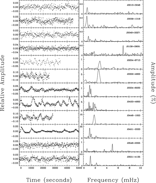
Light curves for every new ZZ Ceti star and possible pulsator in our sample are presented in Figure 7. A quick examination of these results reveals a rich variety of short- and long-period pulsators. In general, the long-period variables tend to have the largest amplitudes, but this is not always the case (see, e.g., J1058+5132). We also find triangular-shaped pulsations, indicative of the presence of harmonics, as well as a few cases of beats, which reveal the presence of closely spaced oscillation modes. The variability of most objects displayed in Figure 7 can be clearly assessed based on the light curves alone, but some require a more quantitative inspection. To this end, the Lomb–Scargle periodograms are shown next to each light curve in Figure 7, covering a frequency spectrum ranging from 0.01 mHz up to 10.5 mHz. The region covering 10.5 mHz up to the Nyquist frequency (50 mHz for a 10 s sampling time) is always consistent with noise and is therefore not shown.
Download figure:
Standard image High-resolution image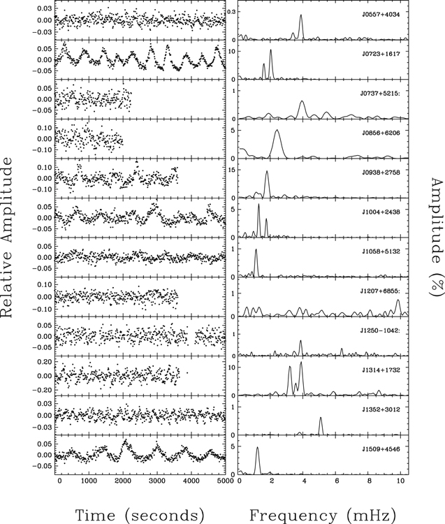
Download figure:
Standard image High-resolution image
Download figure:
Standard image High-resolution image
Figure 7. Light curves and Lomb–Scargle periodograms for the newly discovered ZZ Ceti white dwarfs and possible pulsators. The periodogram amplitude is expressed in terms of the percentage variations about the mean brightness of the star.
Download figure:
Standard image High-resolution imageTo estimate the chance that the detected signals are real, we calculate the false alarm probability (FAP) using the bootstrap method described in VanderPlas (2018). If the dominant periodic signal can be verified by eye and/or has a FAP smaller than 0.1%, we then consider the object as a new variable white dwarf. Objects that fail this criterion but that nevertheless show a periodic signal with an amplitude larger than five times the mean of the entire periodogram are classified as possible pulsators. The two quantities used for classification are included in Table 3, and possible pulsators are identified with a colon in both Table 3 and Figure 7. These objects mostly correspond to candidates located close to the edges of the instability strip, which are expected to show small amplitudes, thus making their variability more difficult to detect. Some of these signals might be buried by the noise of sub-optimal observing conditions, while some might simply be near or below our observational limits. We further discuss our possible pulsators in Section 4.4.
The difference in quality between filtered and unfiltered light curves can be appreciated by comparing J0302+4800 and J0551+4135 in Figure 7. Both have similar Gaia magnitudes and seeing—G ∼ 16.33 and 16.37, FWHM ∼5.8 and 6.0, respectively—but the first has been observed with the g' filter, while the latter has been observed in white light. The pulsations for the object observed in white light are much more obvious, even though it is a shorter-period and smaller-amplitude pulsator than the object observed with a filter.
NOV targets in our sample, as well as the 18 additional objects above the blue edge, are listed in Table 4 with the same information as before, in addition to the photometric precision limit of each light curve and literature identifying the object as a DA, if available. The precision limit corresponds to the standard deviation of the light curve, and is a good indicator of the smallest detectable amplitude in the context of short (< 2 h) light curves. Also included in Table 4 is a column indicating whether or not the object is located within the photometric instability strip, to help distinguish objects from our prior selection based on the spectroscopic instability strip.
Table 4. NOV Candidate Properties
| WD | Gaia DR2 Source | R.A. | Decl. | Phot. Strip |

|
M | G | u | Precision | DA Classification |
|---|---|---|---|---|---|---|---|---|---|---|
| (J2015.5) | (J2015.5) | (K) | ( ) ) |
(%) | ||||||
| J0031+1239 | 2778812676229535616 | 00:31:51.29 | +12:39:45.04 | No | 12,005 ± 91 | 0.577 ± 0.008 | 16.4 | 16.7a | 1.8 | ⋯ |
| J0036+4356 | 387724053774415104 | 00:36:20.14 | +43:56:55.76 | Yes | 11,480 ± 54 | 0.591 ± 0.009 | 16.7 | ⋯ | 1.5 | ⋯ |
| J0037+5118 | 415684119076509056 | 00:37:15.30 | +51:18:44.34 | No | 12,421 ± 113 | 0.790 ± 0.011 | 17.0 | ⋯ | 1.8 | ⋯ |
| J0056+4410 | 377231345590861824 | 00:56:56.67 | +44:10:29.62 | Yes | 11,004 ± 66 | 0.655 ± 0.008 | 16.4 | 16.7a | 1.5 | ⋯ |
| J0056+4410 | 377231139432432384 | 00:56:57.17 | +44:10:18.55 | Yes | 11,798 ± 75 | 0.568 ± 0.006 | 16.0 | 16.3a | 1.5 | ⋯ |
| J0135+5722 | 412839403319209600 | 01:35:17.69 | +57:22:47.67 | Yes | 12,576 ± 89 | 1.156 ± 0.004 | 16.7 | 16.8a | 7.8 | Kilic et al. (2020) |
| J0307+3157 | 135715232773818368 | 03:07:41.88 | +31:57:34.26 | Yes | 11,560 ± 51 | 0.587 ± 0.009 | 16.4 | 16.8b | 1.8 | Kawka & Vennes (2006) |
| J0341−0322 | 3249740657527506048 | 03:41:54.43 | −03:22:39.46 | Yes | 11,804 ± 92 | 0.611 ± 0.006 | 15.3 | ⋯ | 0.9 | Gianninas et al. (2011) |
| J0345+1940 | 63054590968017408 | 03:45:12.05 | +19:40:24.30 | No | 12,367 ± 82 | 0.743 ± 0.004 | 14.2 | ⋯ | 0.7 | ⋯ |
| J0408+2323 | 53716846734195328 | 04:08:03.02 | +23:23:42.48 | Yes | 12,071 ± 110 | 1.038 ± 0.012 | 17.3 | ⋯ | 5.6 | ⋯ |
| J0501+3323 | 184735992329821312 | 05:01:42.72 | +33:23:44.46 | No | 12,107 ± 90 | 0.633 ± 0.008 | 16.1 | ⋯ | 1.4 | ⋯ |
| J0533+6057 | 283096760659311744 | 05:33:45.33 | +60:57:50.14 | Yes | 11,468 ± 61 | 0.585 ± 0.006 | 15.8 | 16.1a | 1.4 | Kleinman et al. (2013) |
| J0538+3212 | 3447991090873280000 | 05:38:58.04 | +32:12:28.39 | Yes | 12,457 ± 154 | 0.996 ± 0.012 | 17.5 | ⋯ | 5.1 | ⋯ |
| J0626+3213 | 3439162768415866112 | 06:26:13.28 | +32:13:11.33 | Yes | 11,660 ± 94 | 0.563 ± 0.007 | 16.2 | ⋯ | 2.5 | ⋯ |
| J0634+3848 | 945007674022721280 | 06:34:16.58 | +38:48:55.09 | Yes | 12,210 ± 106 | 0.926 ± 0.008 | 15.8 | ⋯ | 2.3 | Guo et al. (2015) |
| J0657+7341 | 1114813977776610944 | 06:57:11.11 | +73:41:44.62 | Yes | 12,625 ± 118 | 1.142 ± 0.008 | 17.7 | ⋯ | 3.9 | ⋯ |
| J0717+6214 | 1087442842689746048 | 07:17:07.39 | +62:14:07.53 | Yes | 11,222 ± 67 | 0.648 ± 0.007 | 15.8 | ⋯ | 3.8 | Mickaelian & Sinamyan (2010) |
| J0739+2008 | 672816969200760064 | 07:39:19.79 | +20:08:29.53 | No | 12,283 ± 145 | 0.710 ± 0.009 | 16.0 | 16.2a | 2.8 | ⋯ |
| J0748−0323 | 3080844435869554176 | 07:48:41.91 | −03:23:34.81 | Yes | 11,391 ± 29 | 0.611 ± 0.004 | 15.7 | ⋯ | 1.3 | ⋯ |
| J0751+1120 | 3150770626615542784 | 07:51:41.46 | +11:20:29.07 | Yes | 11,728 ± 58 | 0.558 ± 0.007 | 16.4 | 16.8a | 2.6 | Kilic et al. (2020) |
| J1157+5110 | 791138993175412480 | 11:57:22.38 | +51:10:13.11 | No | 12,075 ± 121 | 0.597 ± 0.008 | 16.3 | 16.7a | 2.3 | ⋯ |
| J1243+4805 | 1543370904111505408 | 12:43:41.62 | +48:05:34.94 | Yes | 12,716 ± 91 | 0.966 ± 0.006 | 17.0 | 17.2a | 4.0 | ⋯ |
| J1308+5754 | 1566530913957066240 | 13:08:48.48 | +57:54:37.03 | Yes | 11,622 ± 83 | 0.704 ± 0.010 | 16.8 | 17.2a | 4.3 | Kilic et al. (2020) |
| J1322+0757 | 3719371829283488768 | 13:22:47.58 | +07:57:29.60 | No | 12,460 ± 67 | 0.702 ± 0.008 | 16.4 | 16.7a | 3.4 | ⋯ |
| J1557−0701 | 4349734833473621248 | 15:57:26.24 | −07:01:21.23 | Yes | 11,792 ± 72 | 0.607 ± 0.006 | 16.1 | ⋯ | 2.7 | ⋯ |
| J1559+2635 | 1316268323580640256 | 15:59:55.25 | +26:35:19.06 | No | 12,266 ± 114 | 0.706 ± 0.007 | 16.3 | 16.6a | 2.6 | ⋯ |
| J1607+2933 | 1317275544951049472 | 16:07:24.37 | +29:33:23.51 | Yes | 10,897 ± 38 | 0.685 ± 0.004 | 15.6 | 16.0a | 0.8 | Stephenson et al. (1992) |
| J1617+1129 | 4454017257893306496 | 16:17:09.38 | +11:29:01.43 | Yes | 11,696 ± 64 | 0.711 ± 0.007 | 16.5 | 16.8a | 0.9 | Pauli et al. (2006) |
| J1626+2533 | 1304081783374935680 | 16:26:59.55 | +25:33:27.60 | No | 13,313 ± 203 | 1.143 ± 0.007 | 17.6 | 17.7a | 5.8 | ⋯ |
| J1635+5053 | 1411867767238390912 | 16:35:05.49 | +50:53:59.78 | Yes | 10,416 ± 41 | 0.554 ± 0.005 | 16.3 | 16.7a | 1.0 | Kilic et al. (2020) |
| J1643−0953 | 4337833650892408448 | 16:43:15.16 | −09:53:05.43 | Yes | 11,443 ± 81 | 0.477 ± 0.008 | 16.5 | ⋯ | 1.7 | ⋯ |
| J1643+6328 | 1631796309274519040 | 16:43:50.51 | +63:28:29.16 | Yes | 12,380 ± 121 | 0.838 ± 0.008 | 17.0 | 17.2a | 1.2 | Kilic et al. (2020) |
| J1643+1118 | 4447022061837071744 | 16:43:54.06 | +11:18:49.28 | No | 12,302 ± 156 | 0.646 ± 0.009 | 16.5 | 16.7a | 2.4 | ⋯ |
| J1652+4110 | 1353302001211658368 | 16:52:00.69 | +41:10:31.36 | Yes | 11,124 ± 76 | 0.894 ± 0.008 | 17.1 | 17.4a | 1.2 | ⋯ |
| J1702+3905 | 1353355434900703616 | 17:02:41.82 | +39:05:58.25 | Yes | 10,547 ± 44 | 0.681 ± 0.005 | 16.3 | 16.6a | 0.9 | Kilic et al. (2020) |
| J1706−0837 | 4336571785203401472 | 17:06:18.45 | −08:37:52.44 | Yes | 12,143 ± 249 | 1.163 ± 0.011 | 17.4 | ⋯ | 4.2 | ⋯ |
| J1728+2053 | 4555079659441944960 | 17:28:45.69 | +20:53:40.98 | No | 12,017 ± 38 | 0.621 ± 0.007 | 16.7 | 17.0b | 1.0 | ⋯ |
| J1805+1536 | 4498531123585093120 | 18:05:43.90 | +15:36:40.03 | Yes | 11,342 ± 85 | 0.581 ± 0.010 | 16.7 | ⋯ | 1.2 | ⋯ |
| J1813+4427 | 2114985726416563072 | 18:13:01.14 | +44:27:19.05 | Yes | 11,149 ± 90 | 1.098 ± 0.007 | 17.7 | ⋯ | 1.4 | ⋯ |
| J1854+0411 | 4281190419601308672 | 18:54:50.41 | +04:11:26.21 | Yes | 12,472 ± 170 | 0.904 ± 0.012 | 17.3 | ⋯ | 4.4 | ⋯ |
| J1857+3353 | 2092086476924423808 | 18:57:57.29 | +33:53:03.88 | Yes | 10,477 ± 62 | 0.632 ± 0.009 | 16.8 | ⋯ | 1.2 | ⋯ |
| J1910+7334 | 2265100885021724032 | 19:10:43.38 | +73:34:39.06 | No | 13,119 ± 214 | 1.087 ± 0.008 | 17.7 | ⋯ | 2.4 | ⋯ |
| J1928+1526 | 4321498378443922816 | 19:28:14.56 | +15:26:38.51 | Yes | 11,543 ± 136 | 1.002 ± 0.013 | 17.8 | 18.0a | 6.4 | Kilic et al. (2020) |
| J1949+4734 | 2086392484163910656 | 19:49:14.55 | +47:34:45.72 | No | 11,911 ± 88 | 0.570 ± 0.006 | 16.1 | ⋯ | 0.7 | ⋯ |
| J1950+7155 | 2263690864438162944 | 19:50:45.89 | +71:55:40.93 | Yes | 11,451 ± 90 | 0.711 ± 0.008 | 16.7 | ⋯ | 1.1 | Voss et al. (2007) |
| J1954+0848 | 4298401105174809984 | 19:54:49.52 | +08:48:50.54 | Yes | 10,594 ± 77 | 0.640 ± 0.012 | 16.9 | ⋯ | 1.3 | ⋯ |
| J2001+2620 | 1835056216381670272 | 20:01:17.81 | +26:20:21.33 | Yes | 11,643 ± 122 | 0.668 ± 0.010 | 16.9 | ⋯ | 2.7 | ⋯ |
| J2014+8018 | 2292229788249205760 | 20:14:34.37 | +80:18:42.53 | Yes | 10,591 ± 62 | 0.668 ± 0.007 | 16.5 | ⋯ | 1.0 | ⋯ |
| J2017+4653 | 2083300584444566016 | 20:17:53.54 | +46:53:14.89 | No | 12,141 ± 108 | 0.600 ± 0.008 | 16.6 | ⋯ | 1.6 | ⋯ |
| J2030+1857 | 1815614965310875520 | 20:30:08.62 | +18:57:34.75 | Yes | 10,511 ± 61 | 0.648 ± 0.009 | 16.7 | ⋯ | 1.3 | ⋯ |
| J2032+4801 | 2083661675243196544 | 20:32:28.75 | +48:01:46.28 | Yes | 11,939 ± 74 | 0.779 ± 0.006 | 16.6 | ⋯ | 0.9 | ⋯ |
| J2045+3844 | 2063435712171048704 | 20:45:28.02 | +38:44:26.65 | Yes | 10,629 ± 43 | 0.649 ± 0.006 | 15.8 | ⋯ | 2.2 | ⋯ |
| J2049+4500 | 2163226700308494080 | 20:49:02.69 | +45:00:36.26 | Yes | 10,993 ± 73 | 0.659 ± 0.007 | 15.6 | 15.9a | 0.6 | Kilic et al. (2020) |
| J2053+2705 | 1845487489350432128 | 20:53:51.74 | +27:05:53.58 | Yes | 11,178 ± 202 | 1.205 ± 0.011 | 18.3 | ⋯ | 2.0 | ⋯ |
| J2054+2427 | 1842670231320998016 | 20:54:46.68 | +24:27:29.23 | No | 12,534 ± 95 | 0.713 ± 0.006 | 15.9 | 16.1a | 1.0 | ⋯ |
| J2119+4206 | 1968901145520461568 | 21:19:01.61 | +42:06:16.46 | Yes | 11,009 ± 102 | 0.450 ± 0.009 | 16.5 | ⋯ | 0.9 | ⋯ |
| J2122+6600 | 2220815923910913920 | 21:22:31.89 | +66:00:42.62 | Yes | 10,613 ± 55 | 0.708 ± 0.006 | 15.9 | ⋯ | 0.7 | ⋯ |
| J2150+2205 | 1793328410074430464 | 21:50:07.49 | +22:05:56.32 | No | 12,761 ± 113 | 0.856 ± 0.010 | 17.0 | 17.2a | 1.2 | ⋯ |
| J2305+5125 | 1995097319287822080 | 23:05:31.71 | +51:25:20.49 | Yes | 11,458 ± 52 | 0.608 ± 0.005 | 15.7 | ⋯ | 2.3 | ⋯ |
| J2312+4206 | 1930609656643838080 | 23:12:42.51 | +42:06:00.42 | Yes | 10,445 ± 62 | 0.574 ± 0.009 | 16.8 | ⋯ | 1.1 | ⋯ |
| J2318+1236 | 2811321837744375936 | 23:18:45.10 | +12:36:02.77 | Yes | 11,710 ± 67 | 0.866 ± 0.005 | 15.4 | 15.7a | 0.6 | Ferrario et al. (2015) |
| J2336+0335 | 2647884790098989568 | 23:36:17.00 | +03:35:08.12 | Yes | 11,218 ± 83 | 0.549 ± 0.010 | 16.5 | 16.9a | 3.2 | ⋯ |
| J2341+5750 | 1998740551069600128 | 23:41:07.61 | +57:50:53.83 | No | 11,793 ± 64 | 0.523 ± 0.005 | 15.8 | ⋯ | 1.0 | ⋯ |
| J2347+5312 | 1993426577008368640 | 23:47:09.28 | +53:12:17.32 | Yes | 10,639 ± 89 | 0.741 ± 0.011 | 17.0 | ⋯ | 1.2 | ⋯ |
| J2356+0803 | 2746936704565640064 | 23:56:06.84 | +08:03:22.28 | No | 12,030 ± 88 | 0.613 ± 0.008 | 16.1 | 16.4a | 1.1 | ⋯ |
Notes.
aSDSS photometry. bCFIS photometry.4.2. The Empirical ZZ Ceti Instability Strip
The M– distribution for the 173 ZZ Ceti candidates and the 18 objects previously selected for high-speed photometric follow-up is shown in the top panel of Figure 8, along with the spectroscopic and photometric instability strips discussed in Section 2. The new ZZ Ceti stars, possible pulsators, NOV objects, and remaining candidates yet to be observed are identified with different symbols in the figure. A first obvious result is the presence of a large number of NOV white dwarfs within the ZZ Ceti instability strip, suggesting that the strip is not pure. We postpone our discussion of these objects to Section 4.3.

Figure 8. Top: M– distribution for the 173 ZZ Ceti candidates and 18 objects previously selected for high-speed photometric follow-up. Different symbols are used to indicate new ZZ Ceti stars (red circles), possible pulsators (black circles), NOV objects (white circles), and remaining candidates yet to be observed (cross symbols). The empirical spectroscopic (dashed lines) and photometric (solid lines) ZZ Ceti instability strips taken from Figure 4 are also reproduced. Bottom: same as top panel, but with the addition of the previously known ZZ Ceti stars within 100 pc from the Sun (magenta circles); for clarity, only the photometric instability strip and observed candidates are shown.
Download figure:
Standard image High-resolution imageIn the bottom panel of Figure 8, we show the same distribution of objects in the M– diagram, but this time we also include the previously known ZZ Ceti pulsators within 100 pc from the Sun, already displayed in the bottom panel of Figure 4. To get a clearer picture, we removed from this figure the location of the empirical spectroscopic instability strip. So far, all of our new ZZ Ceti stars are found well within the previously defined empirical photometric instability strip, with the bulk of them located near the average mass of white dwarfs around ∼0.6
  . More interestingly, we have identified 11 new massive (M ≳ 0.75
  ) pulsators, bringing a noticeable addition to the seven currently known massive ZZ Ceti stars (Córsico et al. 2019) contained within the volume of our sample. The relatively small number of previously known massive pulsators can be attributed to a well-known observational bias. Indeed, ZZ Ceti stars have been previously identified mostly from magnitude-limited surveys. In such surveys, massive white dwarfs are usually underrepresented due to their intrinsically smaller radii and lower luminosities than their normal-mass counterparts (Giammichele et al. 2012). In contrast, our volume-limited survey provides instead an unbiased sample where completeness issues are better controlled.
For similar reasons, less massive white dwarfs, with their larger radii and higher luminosities, will be sampled at much larger distances in magnitude-limited surveys, and will thus be overrepresented. This can be appreciated by comparing the number of low-mass (M ≲ 0.4  ) white dwarfs in Figure 8 with the number observed in Figure 11 of Bergeron et al. (2019), which is based on the white dwarfs contained in the MWDD, most of which have been discovered in magnitude-limited surveys. Hence, not surprisingly, our survey has revealed no additional low-mass pulsators. The only previously known low-mass ZZ Ceti star in Figure 8 is HS 1824+6000 (Steinfadt et al. 2008), whose spectroscopic mass (3D-corrected) is also low, M ∼ 0.45
  according to Gianninas et al. (2011).
Also worth mentioning is our discovery of two new ultramassive (
 ) pulsators, J0551+4135 (1.127 ± 0.005
  ) and J0204+8713 (1.049 ± 0.0015
  ). At the time of writing this paper, only three other ultramassive ZZ Ceti stars have been confirmed: BPM 37093 with M ∼ 1.1
  (Kanaan et al. 1992), SDSS J084021.23+522217.4 with M ∼ 1.16
  (Curd et al. 2017), and GD 518 with M ∼ 1.24
  (Hermes et al. 2013). Our new massive and ultramassive pulsators represent objects of interest for asteroseismological studies of the process of core crystallization within the instability strip (Romero et al. 2013). J0551+4135 is of particular interest since ultramassive ZZ Ceti stars with
 are expected to have a very large portion of their mass in the crystallized phase (De Gerónimo et al. 2019), and observations with 2 minute cadence from Transiting Exoplanet Survey Satellite (TESS, Ricker et al. 2015) are available for this object.
We end this section with a few words regarding the exact location of the empirical ZZ Ceti instability strip based on our photometric survey. The bottom panel of Figure 8 shows all variable stars, both new and known, to be within the photometric instability strip previously defined in Figure 4, within the uncertainties. Moreover, new pulsators found near the red edge of the strip show diminishing amplitudes as they approach the edge itself (further discussed in Section 4.4), strengthening our assumption of its location. By the same token, the 18 NOV objects observed above the blue edge are particularly useful to pinpoint its exact location. Given the results shown here, we do not feel it is necessary to revise the location of the blue edge of the photometric instability strip. This in turn suggests an excellent internal consistency between the spectroscopic and photometric determinations, with the understanding that one is shifted in temperature with respect to the other.
4.3. Non-variability and the Purity of the ZZ Ceti Instability Strip
In this section, we discuss the purity of the ZZ Ceti instability strip with respect to our findings, summarized in the top panel of Figure 8. There are several aspects to consider when assessing the purity of the instability strip, the most important of which are the precision limits of the high-speed photometric observations, and the accuracy and precision of the physical parameter measurements.7 In our case, we also have to consider the atmospheric composition of the candidates.
We find in our survey 47 NOV white dwarfs within the photometric instability strip, nine of which have a DA spectral type published in the literature, while eight more have recently been confirmed to be DAs by Kilic et al. (2020). We note, however, that two of the published DA spectral classifications are dubious. J0717+6214 (GD 449) was classified as "DA:" by Mickaelian & Sinamyan (2010), where the colon implies an uncertain spectral type. It would be difficult to misclassify such a bright (G ∼ 15.8) DA star in the temperature range where ZZ Ceti stars are found, given that the Balmer lines reach their maximum strength around  K. We suspect the authors may have detected an Hα absorption feature in a helium-rich DBA white dwarf. The second object, J1950+7155 (HS 1951+7147), is classified as DA in Simbad, with a reference to Voss et al. (2007), who reported this object to be a non-variable white dwarf in their Table 1. The atmospheric parameters for this object were derived from BUSCA photometry using pure hydrogen models (see Voss et al. for details), although we find no evidence for a firm DA spectral classification in their analysis. In fact, there was no follow-up on HS 1951+7147 in the spectroscopic analysis of DA white dwarfs from the ESO SN Ia Progenitor Survey published by Koester et al. (2009). As there is no spectroscopic evidence for the DA classification for this object, the possibility of a helium atmosphere remains.
We also realized after the fact that J2318+1236 (KUV 23162+1220) is a highly magnetic (Bp ∼ 45 MG) DA white dwarf (Ferrario et al. 2015, see the spectrum in Figure 5 of Gianninas et al. 2011). It has been suggested that the presence of a strong magnetic field might have a dramatic effect on the driving mechanism of the pulsations (see Section 3.4 of Tremblay et al. 2015). This suggestion has been reinforced by Gentile Fusillo et al. (2018), who reported the convincing case of a  K DA white dwarf (WD 2105−820, L24-52) in which atmospheric convection has been suppressed by the presence of even a weak magnetic field (Bp ∼ 56 kG, Landstreet et al. 2012). Since the driving mechanism in ZZ Ceti stars is located at the bottom of the hydrogen convective zone, it is reasonable to assume that magnetic DA stars should not pulsate. Our photometric observations of J2318+1236 certainly support this interpretation. It is thus possible that additional NOV objects in our sample are magnetic DA white dwarfs, even weakly magnetic.
Among the 47 NOV white dwarfs within the instability strip, 18 are confirmed to be hydrogen-rich through their u-band photometry (9 of these 18 also have a firm DA spectral type, including the magnetic DA). Excluding the genuine DA stars discussed above, this leaves 26 NOV white dwarfs within the strip that could possibly have a helium atmosphere or be magnetic; these can only be confirmed with additional spectroscopic or u-band photometric observations. We thus end up with 20 NOV white dwarfs within the instability strip that either are hydrogen-rich through their u-band photometry or are classified as genuine DA stars, excluding the magnetic white dwarf. These are the offending NOV objects we need to explain. In every case, there is always the remote possibility for pulsations in a ZZ Ceti star to be hidden from us due to geometric considerations (see, for example, HS 1612+5528 discussed in Gianninas et al. 2011).
While Bergeron et al. (2004) argued that the ZZ Ceti instability strip is pure—i.e., devoid of non-variable white dwarfs—when analyzed using the spectroscopic technique, our study is the first assessment of its purity based on the detailed photometric approach. Genest-Beaulieu & Bergeron (2019, see also Gentile Fusillo et al. 2019; Tremblay et al. 2019) discussed at length the accuracy and precision of both the spectroscopic and photometric techniques. They argued that even though the photometric approach yields physical parameters that are more accurate, the spectroscopic method is probably more precise. For instance, while differences in spectroscopic and photometric temperatures in Figure 5 are of the order of 5% or less, on average, there are cases where these differences can reach 15% or more.
We can explore these discrepancies more quantitatively by comparing our photometric parameters with those obtained from spectroscopy for some of the offending NOV objects within the instability strip with optical spectra available to us. For instance, for J0341−0322 (LP 653-26; spectrum from Gianninas et al. 2011) we obtain a spectroscopic temperature of Tspec = 12,807 K using our ML2/α = 0.7 models, a value 8.5% higher than our photometric temperature given in Table 4 ( K). With a (3D-corrected) spectroscopic mass of 0.64
  , this white dwarf is thus located above the empirical spectroscopic instability strip. Similarly, we find that J0533+6057 (SDSS J053345.32+605750.3; spectrum from Kleinman et al. 2013) and J1617+1129 (HS 1614+1136; spectrum from Koester et al. 2009) have spectroscopic temperatures of Tspec = 13,130 K (with
  K) and Tspec = 13,970 K (with
  K), respectively, both significantly above the spectroscopic instability strip. An even more extreme case is that of J1243+4805 (HS 1241+4821; SDSS spectrum from Kleinman et al. 2013), for which we obtain Tspec = 14,838 K, a value more than 2000 K hotter than our photometric temperature of
  K. Finally, Kawka & Vennes (2006) report a spectroscopic temperature of Tspec = 13,300 K for J0307+3157 (NLTT 9933), while we obtain Tphot = 11,560 K. Hence, most of the spectroscopic temperatures push these NOV objects above the blue edge of the spectroscopic instability strip, suggesting that the photometric temperatures might sometimes be underestimated.
It is worth noting in this context that among the new ZZ Ceti stars listed in Table 3, 19 are known to be DA white dwarfs. Limoges et al. (2015) obtained spectroscopic parameters ( and M) for three of those DA stars (J10042+2438, J19033+6035, and J18435+2740) that place them well within the ZZ Ceti instability strip. We also have spectra for 13 DA stars from the analysis of Kilic et al. (2020), and even though most of these are classification spectra with low signal-to-noise ratios, the spectroscopic parameters obtained from the best quality spectra also place them within the strip. This reinforces the idea that the NOV objects discussed above represent cases where the photometric parameters suffer from large errors.
Also, we cannot exclude that in some cases the differences between spectroscopic and photometric temperatures may be explained in terms of unresolved double degenerate binaries. Indeed, Bergeron et al. (2018) showed that the most extreme differences in physical parameters ( and M) tend to be associated with double DA white dwarf binaries, for which the measured radii inferred from the photometric technique are overestimated—and thus the masses are underestimated—due to the presence of two stars, while the spectroscopic masses remain relatively unaffected. J2119+4206, our lowest-mass NOV candidate, seems to be such a case. It is also possible to have an unresolved double DA+DC binary, where the DC star dilutes the hydrogen lines of the DA component of the system, making the object appear as a massive DA white dwarf when analyzed with the spectroscopic technique. An excellent example is the DA star G122-31—also discussed by Bergeron et al. (2018)—which Harris et al. (2013) reported as being an unresolved degenerate binary. The spectroscopic parameters for this object are
  K and
K and  (or M = 1.19
  ), while the photometric values are significantly different,
  K and
K and  (or M = 0.95
  ).
).
The bottom line of the above discussion is that we need a combined spectroscopic and photometric investigation of our NOV candidates for any serious discussion of the purity of the ZZ Ceti instability strip. Therefore we cannot conclude at this stage that the strip contains a significant number of non-variable DA white dwarfs.
Finally, we look at the confirmed ZZ Ceti stars to estimate the likelihood of pulsations being hidden within photometric noise for the NOV candidates. As discussed in the next section, pulsators located very close to the edges of the instability strip typically show the smallest amplitudes, sometimes as small as 0.1%. Given that our typical photometric precision is about 3.4% for the average Gaia magnitude  of our sample, detecting such small pulsations in fainter objects is unlikely with our observational capabilities. As we move further away from the edges and toward the center of the strip, ZZ Ceti stars tend to have larger amplitudes, and the likelihood of pulsations being smaller than our photometric precision limit decreases. Another possibility is to have observed the candidate amid a beat caused by two or more oscillation modes interfering destructively with each other. For example, in the case of J0324+6020 (see the light curve in Figure 7), we observed a beat lasting well over an hour, during which the pulsation amplitude drops to a nearly undetectable level. For fainter candidates, this could easily translate into observing no pulsations. Ultimately, our NOV candidates will have to be reobserved with better precision to better constrain their non-variability. Longer light curves would also be more sensitive to small-amplitude pulsations. In particular, candidates located near the edges will require higher-performance facilities, or longer observations, than those offered at the Mont-Mégantic Observatory.
4.4. Pulsational Properties
ZZ Ceti white dwarfs exhibit a wide variety of light curves, and the investigation of their periods, amplitudes, and nonlinearities can reveal a wealth of information in the context of asteroseismological studies. Of particular interest in this section is how these characteristics evolve empirically across the ZZ Ceti instability strip. Many global patterns have been established some time ago (Robinson 1979; Fontaine et al. 1982), such as the inverse correlation between effective temperature and period (Winget & Fontaine 1982). A temperature–amplitude relationship was also discussed by Kanaan et al. (2002) and Mukadam et al. (2006). In particular, Mukadam et al. have shown that the amplitudes increase with decreasing  , reaching a maximum near the cooler half of the strip, after which the amplitudes start to drop toward the red edge. While these temperature-dependent relations have proven to hold true, it has been demonstrated since then that they also depend on surface gravity (Fontaine & Brassard 2008). More recently, Hermes et al. (2017) analyzed a sample of 27 ZZ Ceti stars using the space-based observations taken by the Kepler telescope. The extended duration of the light curves allowed confirmation of what appears to be a new phase in the evolution of DAVs as they cool past the center of the instability strip: aperiodic outbursts increasing the mean stellar flux by a few per cent to 15%, over several hours, and recurring sporadically on a timescale of days. Here, we take a fresh look at the ZZ Ceti ensemble characteristics using our sample of new pulsators.
Figure 9 shows a color map in the M– plane for the dominant periods (Pd) present in the light curves of our new and possible pulsators, where the size of every symbol scales according to the amplitude of the object's dominant period. Also included in the figure are a few previously known ZZ Ceti stars of interest, which will be discussed below. We detect periods between 195 and 1600 s, with a clear evolution from small periods near the blue edge of the strip to longer values as we approach the red edge, with a few exceptions: the two ultramassive pulsators and two other objects near the red edge. These will be discussed further below. Massive (M ≳ 0.75
  ) pulsators also follow the general trend, although most of their periods are found within a narrow range from 350 to 600 s. In the first studies of the ensemble characteristics of massive ZZ Ceti white dwarfs, Castanheira et al. (2013) suggested a mode selection mechanism preventing periods around 500 s because of a lack of observed pulsations near this value (see their Figure 5). While mode trapping is predicted to be more important for massive pulsators (Brassard et al. 1992), our results go against the idea of a particular phenomenon completely suppressing periods between 400 and 600 s.
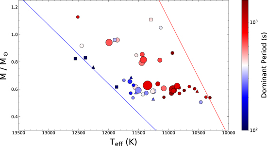
Figure 9. Logarithmic color map of the dominant periods in the M– plane for our new ZZ Ceti white dwarfs (circles) and possible pulsators (triangles). Also displayed are a few previously known ZZ Ceti stars (squares) discussed in the text. The size of every object gives a measure of the amplitude of their dominant period, linearly scaling from 0.05% to 30%.
Download figure:
Standard image High-resolution imageThe odd pulsator J2319+2728, located close to the cool edge of the ZZ Ceti instability strip at M ∼ 0.5  , seemingly stands out from the general trend of increasing periods, with Pd = 277 s. A similar object (SDSS J2350−0054) was reported by Mukadam et al. (2004), who found no obvious explanation for its peculiar properties. In the case of J2319+2728, the Pan-STARRS photometry was found to possibly be contaminated by a neighboring luminous star, which most likely results in an overestimation of the stellar radius—and thus an underestimation of the stellar mass—when using the photometric technique. The impact on
  is presumably less important, given that this ZZ Ceti star is still located within the boundaries of the instability strip, but the temperature remains affected nonetheless. Given its pulsational properties, we suspect the object actually lies among the bulk of our new pulsators, closer to the blue edge.
Another noteworthy case is the ultramassive pulsators. J0551+4135 shows a period (Pd = 809 s) much longer than the periods found in other massive ZZ Ceti stars in the same temperature range, and J0204+8713 shows the exact opposite with a much shorter period (Pd = 330 s) than found in cool massive pulsators. As an attempt to discern a trend among the ultramassive pulsators in the M–  plane, we included in the color map of Figure 9 two of the three aforementioned ultramassive objects, using our own photometric measurements of their Pan-STARRS photometry (see Section 4.2). With GD 518 at
  K and M = 1.108
  (Pd ∼ 442 s, Hermes et al. 2013), SDSS J084021.23+522217.4 at
  K and M = 0.962
  8
(Pd ∼ 326 s, Curd et al. 2017), the four ultramassive ZZ Ceti stars appear to show diminishing periods as they cool down the strip. A more detailed study of these objects will be required to confirm this phenomenon, because it would go against the general trend observed in all other ZZ Ceti white dwarfs.
8
(Pd ∼ 326 s, Curd et al. 2017), the four ultramassive ZZ Ceti stars appear to show diminishing periods as they cool down the strip. A more detailed study of these objects will be required to confirm this phenomenon, because it would go against the general trend observed in all other ZZ Ceti white dwarfs.
Next, we look for a correlation between the amplitude and the dominant period using the ZZ Ceti stars discovered in our sample. The results, displayed in Figure 10, reveal amplitudes varying from 0.2% to 35%, wherein shorter periods show smaller amplitudes, followed by an increase in amplitude until the dominant period reaches ∼800 s, above which point the amplitudes start diminishing. Our massive ZZ Ceti stars seem to follow the same overall trend as their normal-mass counterparts. Incidentally, this trend can be seen in the M– plane of Figure 9, where amplitudes are at their highest at the center of the strip, then diminish as the pulsators move toward the edges. For our pulsators, higher amplitudes also tend to coincide with light curves showing more complex features. Overall, the ensemble characteristics observed here agree with those established in the literature. We did not, however, detect any outburst events such as those described in Hermes et al. (2017). This comes as no surprise because these events are known to last several hours, while our observations were generally shorter than 2 hr.

Figure 10. Logarithm of the amplitude (in %) against the dominant period for the new ZZ Ceti white dwarfs (red dots) and possible pulsators (black dots) in our sample; massive (M > 0.75  ) ZZ Ceti stars are shown as green dots.
Download figure:
Standard image High-resolution imageWe finish this section with a discussion regarding the authenticity of our so-called possible pulsators. We compare their physical and pulsational properties with those of the new ZZ Ceti stars in our sample, starting with the warmest object. We have also included three known ZZ Ceti stars in Figure 9, located extremely close to the blue edge of the instability strip, to make up for the lack of new pulsators within that region. These three known ZZ Ceti possess some of the shortest periods and smallest amplitudes ever detected: HS 1531+7436 with Pd ∼ 111 s and an amplitude of ∼4 mma (millimodulation amplitude) (Voss et al. 2006), GD 133 with Pd ∼ 120 s and an amplitude of ∼4 mma (Silvotti et al. 2006), and G226-29 with  and an amplitude of ∼1 mma (Kepler et al. 1983). The last two are relatively bright—with Gaia magnitudes G = 14.76 and 12.29, respectively—and their pulsations might not have been detected if not for this. For instance, G226-29 had been observed several times with telescopes as large as 1.6 m, but its variability could not be confirmed until observations were secured with the 6.5 m Multiple Mirror Telescope. We thus expect pulsators very close to the blue edge of the strip to have periods around 100 s and very small amplitudes, which is exactly the kind of weak signal we detected in our possible massive pulsator J1207+6855. The rest of the possible pulsators are located around 0.6
  in Figure 9. Their periodograms mostly show peaks within in the expected period range, although the amplitudes are too small to be confirmed unambiguously. Their pulsations also follow the usual period–amplitude trend, as shown in Figure 10. All of our possible pulsators will need to be reobserved with better instruments, or at the very least, under exceptional observing conditions. Space-based surveys (i.e., TESS and the upcoming PLATO 2.0 Mission; Rauer et al. 2014) may offer an interesting avenue to acquire higher-quality data, in particular for brighter objects. Furthermore, these surveys could also be useful for asteroseismic studies of our new ZZ Ceti stars, as well as to verify with greater precision whether NOV candidates are truly non-variable.
5. Conclusion
In this paper, we presented the first study of the photometric ZZ Ceti instability strip using results from the combined Gaia and Pan-STARRS surveys. In addition to searching for new puslators, we aimed to verify whether ZZ Ceti white dwarfs occupy a region of the M– plane where no non-variable stars are found, supporting the idea that ZZ Ceti stars represent a phase through which all hydrogen-atmosphere white dwarfs must evolve.
We first selected all white dwarfs and white dwarf candidates in the Northern Hemisphere within 100 pc of the Sun with parallax measurements from the Gaia Data Release 2 catalog, which we then cross-referenced with the Pan-STARRS Data Release 1. Using the so-called photometric technique, we measured with high precision the physical parameters ( and M) of every object by combining Pan-STARRS grizy photometry with Gaia astrometry. Since the Pan-STARRS photometry alone does not allow for a determination of the chemical composition of white dwarfs, we also included SDSS or CFIS u photometry, when available, in our model atmosphere fits. The u band covers the Balmer jump, which represents a good discriminant between hydrogen- and helium-rich atmosphere white dwarfs, and it can be used efficiently to exclude non-DA stars from our list of ZZ Ceti candidates. To establish a region of the M–
 plane where the DA pulsators could be found, we first applied 3D corrections to the spectroscopic parameters of a sample of bright ZZ Ceti stars. We also made adjustments to the effective temperature of the boundaries of the instability strip to account for the known discrepancies between spectroscopic and photometric parameters, producing our final empirical photometric instability strip. We identified a final sample containing 173 ZZ Ceti candidates within this strip.
We acquired high-speed photometry for a sample of 90 ZZ Ceti candidates within the photometric instability strip using the PESTO instrument attached to the 1.6 m telescope at the Mont-Mégantic Observatory. Among these, 38 proved to be clearly variable, while five show possible small-amplitude pulsations, and 47 were not observed to vary. Additionally, 18 objects near, but above the blue edge of the instability strip, were observed and showed no variability.
The implications of our findings, as well as the nuances of the photometric technique in the context of ZZ Ceti identification, have been discussed at length in this paper. The first remarkable result was, of course, the large number of new ZZ Ceti white dwarfs identified in our study. We discovered 11 massive ZZ Ceti stars (M > 0.75  ), including two very rare ultramassive pulsators, making a significant contribution to the number of such known objects. We attribute this high rate of identification of new massive pulsators to the use of a volume-limited, rather than a magnitude-limited, sample for the selection of our ZZ Ceti candidates. The distribution of our new ZZ Ceti stars in the M–
 plane was shown to be in excellent agreement with our empirical photometric instability strip, suggesting a good internal consistency between the spectroscopic and photometric methods. The pulsation ensemble characteristics of our sample in the M–
 plane were also examined qualitatively, and showed good agreement with the empirical trends previously established. In particular, massive pulsators seemed to follow the same tendencies as their normal-mass counterparts, with the exception of the new ultramassive variable white dwarfs.
We attempted to assess the purity of the instability strip by investigating in depth the candidates showing no variability. Our study turned out to be inadequate for a meaningful discussion of this topic, and it will require further spectroscopic investigations of the non-variable candidates. Observing the candidates located near both boundaries of the strip with higher-performance facilities than those offered by the Mont-Mégantic Observatory will also be necessary in this context, because objects in these regions are known for their very low-amplitude variations, and these are most likely not detectable with our current means. Furthermore, high-speed photometric observations of such objects will eventually allow us to constrain more accurately the exact location of the boundaries of the instability strip.
Finally, it would be interesting to apply this photometric approach to identify new pulsating white dwarfs of different types. DBV stars would make an excellent choice, because they are the most studied class of white dwarf pulsators besides the ZZ Ceti stars.
We thank N. Giammichele for a careful reading of our manuscript and for her constructive comments. We would also like to thank the staff of the Observatoire du Mont-Mégantic for their assistance and for conducting queue mode observations. This work was supported in part by the NSERC Canada and by the Fund FRQ-NT (Québec). This work has made use of data from the European Space Agency (ESA) mission Gaia (https://www.cosmos.esa.int/gaia), processed by the Gaia Data Processing and Analysis Consortium (DPAC, https://www.cosmos.esa.int/web/gaia/dpac/consortium). Funding for the DPAC has been provided by national institutions, in particular the institutions participating in the Gaia Multilateral Agreement. This research has made use of the NASA/IPAC Infrared Science Archive, which is operated by the Jet Propulsion Laboratory, California Institute of Technology, under contract with the National Aeronautics and Space Administration. This work has also made use of data obtained as part of the Canada–France Imaging Survey, a CFHT large program of the National Research Council of Canada and the French Centre National de la Recherche Scientifique. Based on observations obtained with MegaPrime/MegaCam, a joint project of CFHT and CEA Saclay, at the Canada–France–Hawaii Telescope (CFHT), which is operated by the National Research Council (NRC) of Canada, the Institut National des Science de l'Univers of the Centre National de la Recherche Scientifique (CNRS) of France, and the University of Hawaii.
Footnotes
- 1
Note that the algorithm described here is being used for the Pan-STARRS photometry provided in the Montreal White Dwarf Database (MWDD, Dufour et al. 2017).
- 2
It is worth mentioning in the present context that the pure hydrogen model atmospheres—calculated with the ML2/α = 0.7 version of the mixing-length theory—are identical to those used to determine the empirical ZZ Ceti strip based on spectroscopy displayed in Figure 1.
- 3
- 4
- 5
- 6
The WD ID numbers JXXXX+YYYY assigned here are based on the Gaia J2015.5 coordinates.
- 7
Statistically speaking, the precision of the method describes random errors, a measure of statistical variability, repeatability, or reproducibility of the measurement, while the accuracy represents the proximity of the measurements to the true value being measured.
- 8
We note here that the photometric mass for this object is below 1
 . We have optical spectra for two of our new ZZ Ceti stars (from Kilic et al. 2020) with , and although the spectrum of J0856+6206 is too noisy for a proper spectroscopic analysis, we obtain for J1812+4321 a spectroscopic mass of Mspec = 0.99 (compared to Mphot = 0.917 ), possibly adding another ultramassive white dwarf to the sample.


