Several post-processing methods were proposed to overcome the excess noise factor induced by EMCCD multiplication register. Each method has a unique effect on SNR. However, since SNR does not account for photometric accuracy, it cannot be reliably used to directly compare the performance of these algorithms. A normalized quadratic error that accounts for both SNR and accuracy is proposed as an alternative figure of merit. This approach provides a quantitative and rigorous comparison. Using both experimental and simulated frames in the faint-flux range, it is used to compare the existing EMCCD post-processing methods.
Charge-Coupled Devices (CCDs) are widely used for imaging and their sensitivity is acceptable for most applications. However, when light become sparse, which is the case for high frame rate or low lighting applications, the signal-to-noise ratio (SNR) of these devices drops rapidly due to their readout noise. For these faint-flux imaging applications, overcoming the readout noise is essential. The advent of the EMCCD made it possible to break readout noise barrier, rendering single photon detection possible on a CCD focal plane.1
This low readout noise comes at the price of an Excess Noise Factor (ENF) that, from a SNR point of view, has the same effect as if the quantum efficiency of the device were halved.2 Analog Readout (AR), where the signal of the pixel is calculated by simply dividing the output signal by the mean gain of the EM register, is plagued by this reduction in SNR. Authors have proposed methods to circumvent the ENF (Photon Counting,1, 3–6 Thresholding,7 Multiple Thresholding,4 Bayesian Inference7 and Thresholding with Bayesian Inference8 ). By taking into account the main sources of noise affecting the EMCCD (dark current, clock-induced charged, and readout noise), they aimed at best estimating the true input flux on the CCD from the output signal. This paper reviews and compares these post-processing methods.
Since the purpose of these post-processing methods is to most accurately deduce the real input photon flux on a pixel from the digital readout, a proper figure of merit must be chosen to yield a coherent comparison. This figure of merit will be described in section 2. Then, section 3 describes the reviewed post-processing methods, section 4 develops the methodology used to compare the post-processing methods and section 5 presents the interpretation of the NQE figures.
It is commonplace to measure the quality of a signal using the SNR, here defined as the ratio of the mean signal µ over its standard deviation σ.
![]()
It can be quite challenging in practice to apply this general definition to the computation of SNR for postprocessed signals.
This first difficulty comes from the introduction of biases by specific post-processing methods that must be carefully considered in the mathematical description of the variance σ2 . As shown in [9], distinct SNR expressions are obtained for analog readout operation (AR) and photon counting (PC) as the latter prescinds the excess noise factor (ENF). For simple post-processing methods, it is often possible to get a closed-form expression for the SNR. However, as the complexity of the method grows, it becomes more and more difficult to accurately describe the variance and reach a closed-form expression. A second difficulty of using SNR as a figure of merit is that it does not account for the accuracy of the post-processed signal with respect to the true value of the signal. SNR only measures to what extent the information signal exceeds the noise. Hence, it is possible to have a high-SNR post-processed signal which completely misrepresents the original signal.
When comparing various post-processing methods, one is interested in their photometric accuracy. For that purpose, a quadratic error (QE) is used to assess performance. Letting S be the post-processed signal computed from N sample frames and S* be the true signal (assumed constant over the samples), the QE is defined as follows.

In practice, S* is not known but it can be estimated by averaging the raw signal over a large sample (herein set at 1000 frames) to get an approximation called s̅* . This way, one can easily compute the QE using S* ≈ s̅* for any signal produced by any post-processing method. This figure of merit thus bypasses the two main difficulties associated to SNR. (1) Its definition can be applied to any method as it prescinds post-processing particularities. (2) It is able to evaluate the accuracy of the method using s̅* , providing s̅* is calculated from a large enough sample and a constant signal.
2.1 Ideal detector normalization
The QE defined above can be further refined by normalizing it with the QE of an ideal detector subject to shot noise only. Here it is crucial to understand that even such a detector will not lead to a perfect knowledge of the true signal S ? . If λ is the mean flux of the source measured in photons per pixel per frame, the number n of photons reaching one pixel during the integration time of a single frame follows a Poisson distribution characterized by λ. The minimum-variance unbiased estimator

based on N independent observations ni may be used to estimate λ, or equivalently the most probable number of photons to reach a pixel in one frame. Setting S = λˆ and S* = λ in (2), one sees that the result of this QE depends on the particular values of ni . So that this result stays independent from the readouts, all possible outcomes of N observations are averaged. Thus, the averaged QE for the shot noise estimator λˆ is obtained, where E denotes the expectation operator.

Note that the above expression is simply the inverse squared SNR of a Poisson distribution of mean Nλ. QESN is a decreasing function of N and so it confirms the intuition that accuracy of the estimator is increased by using more observations. Equation (4) acts as a normalization factor in the following definition of the normalized quadratic error.

NQE is a positive quantity assessing the performance of a post-processing method normalized to what one would find in the presence of shot noise only. When comparing methods, low NQE and high performance are synonymous.
2.2 Comparison of SNR and NQE
In addition to assessing the accuracy of a method, NQE also gives insight on the performance of postprocessing methods as a function of flux. Figure 1 presents normalized SNR and NQE for the simplest postprocessing methods presented in section 3: Analog readout and Photon counting. They are considered “simple” because the expression of their SNR can be demonstrated analytically
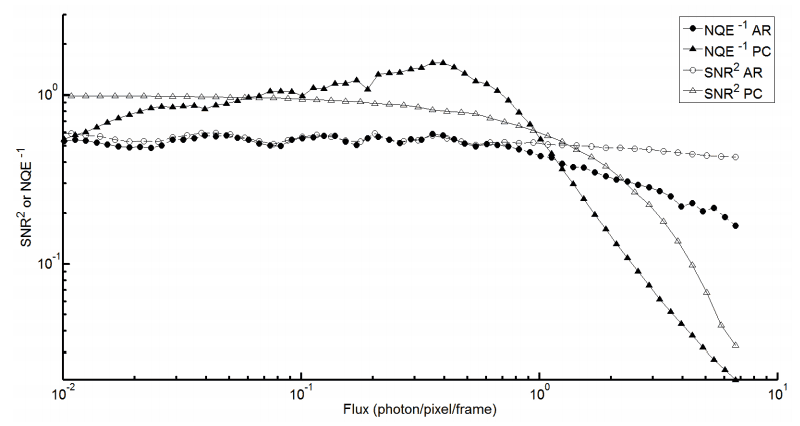
Here squared SNR is compared with inverted NQE to keep the same relative units and order of comparison. Figure 1 shows that both NQE and SNR behave similarly in regards to assessing relative performance of two methods. However, the NQE peak around 0.4 photon/pixel/frame shows that NQE has additional information compared to SNR. This information is characteristic of the photometric accuracy of post-processing methods (see Section 5).
These results show that NQE gives a measure of photometric accuracy in addition to giving information corroborating SNR. This establishes NQE as a more accurate choice for comparing post-processing methods.
This section summarizes the fundamentals of the six post-processing methods compared in this review. Further details are available in the original papers.
3.1 Analog readout (AR)
The AR operation of the EMCCD consists in dividing the raw output signal by the mean gain G of the EM register. It allows more than one photon/pixel/frame to be measured.2 The EM register gain being stochastic, an excess noise factor appears. At high gains, the ENF has the same effect on the SNR as if the quantum efficiency of the EMCCD were halved. An EMCCD operating in AR typically outperforms a low-noise CCD for fluxes lower than ∼5 photons per pixel per frame.9
3.2 Photon counting (PC)
When dealing with extreme faint fluxes, one can expect to measure no more than one photon. Under this assumption, the ENF can be suppressed using photon counting. This method compares the output value to a threshold T. If the output exceeds the threshold, the pixel is set as having collected a single photon. Otherwise, the pixel is assumed empty. Clearly, PC is not intended to support multiple events, leading to coincidence losses when two or more photons reach the same pixel during a single frame. PC also ignores events that are not amplified enough by the EM register and are thus lost in the readout noise due to an output lower than the threshold. On the other side, PC overestimates the input photon flux when readout noise exceeds the threshold. These phenomenon illustrate the importance of an informed threshold choice. For the purpose of this review, this threshold is fixed at five times the readout noise.10 This value is used for subsequent post-processing methods requiring a threshold.
Using N frames, one applies the threshold T to each frame and gets N binary frames whose pixels values yPC,i are either 0 or 1. The estimated flux λˆ is then taken as the mean of these frames.

3.3 Thresholding (T)
Authors of [7] proposed a similar method to PC with slightly different thresholding scheme. Here, the readout noise R of the EMCCD is modeled by a Gaussian distribution with zero mean and variance σ2 . The probability that the readout noise exceeds the threshold T when there is no input photoelectron is given by

where N (x|0, σ2 ) is the probability density function (PDF) of the aforementioned Gaussian and erf(·) is the error function. This probability is used to get an effective number of frames having undergone a photon event and compute the following estimation of the flux

where Q denotes the number of frames among the N samples with a pixel output greater than T. Finally, the correction is assumed small compared to (N −Q)/N and the first-order Taylor expansion ln (a + x) ≈ ln (a)+x/a yields the final result

3.4 Multiple thresholding (MT)
MT4 also uses thresholding to suppress ENF coming from the EM register. In contrast to PC, MT introduces multiple thresholds Tn, n ∈ N, so that when the output of the pixel lies between Tn and Tn+1, it is considered that n photon events occurred during the integration time. The set of Tn are calculated from the probability density function p(y|λ) of the output y of the EMCCD with mean gain G resulting from a mean flux λ.

Equation (10) models the output of the EM register with k input electrons as a gamma distribution characterized by k and G, and the number of input electrons as a Poisson distribution characterized by λ. Setting T0 ≡ 0, the n-th threshold Tn is defined as the output y where the probability density for mean light levels n and n + 1 are equal.
![]()
The solutions of (11) are found numerically and are expressed as fractions of the mean gain G and can be found in [4]. As n increases, Tn approaches n so that for n ≥ 11, the authors set Tn = n.
For mean light fluxes lower than 20 photons per pixel per frame, it is suggested to apply a non-linear photometric correction taking into account the fact that there is a significant probability for a single photon event to be interpreted as a multiple photon event. The correction is given as a function of the result yest of the thresholding step so that the final output yMT of the method is

To get an estimation of the mean input flux from the final outputs yMT,i of N frames, the mean is calculated.

3.5 Bayesian inference (BI)
Authors of [7] also developed a detailed probabilistic description of the various processes of electron generation occuring in an EMCCD. As in MT, the output of the EM register with n input electrons is modeled with a gamma distribution. The effect of clock induced charges (CIC) arising from the parallel register of the CCD (pCIC) and from the serial EM register (sCIC) are also considered. Spurious pCIC electrons, modeled with a Poisson distribution, are generated before the EM register. Hence, they are subject to the whole multiplication process, just as normal photoelectrons. A single spurious sCIC electron generated at a given stage of the EM register is described by an exponential distribution whose parameter is the mean gain associated to the remaining stages of the register. Finally, the readout noise at the end of the EM register is assumed to be a zero-mean Gaussian with variance σ 2 .
Considering an EM register with mean gain G and probability ps for a sCIC electron to be generated at each of the m stages, the authors derive the following expression for the PDF of the output y of the EMCCD associated to an input flux λ

where
![]()
is the mean gain for a spurious electron generated at the k-th stage of the EM register, G(y|k, G) is the PDF of a gamma distribution of parameters k and G and P(k|λ) is the probability mass function of a Poisson distribution of parameter λ. In this review, ps = 10−5 and m = 512 are taken as typical values for these parameters.
Equation (14) is a mixture distribution describing exclusively the following situations: 1) no photoelectron or spurious electron is generated and only readout noise is read; 2) no photoelectron or pCIC electron is generated and a sCIC electron is generated at stage k in the EM register; 3) one or more photoelectrons or pCIC electrons are generated. Note that in cases 2) and 3), the readout noise is assumed negligible and that in case 3), sCIC electrons are not considered.
Being interested in the incoming flux, one can use Bayes’ theorem to inverse the PDF (14) and get p(λ|y).

This inversion requires a prior distribution over λ to be introduced. The authors propose that this prior should not be a peaked function as there is no prior information available as to what value λ should take. Following this reasoning, this review uses a discrete prior over n possible values and assigns to each an equal probability 1/n. As a consequence, the integral in the denominator becomes a sum which can be easily computed. The probability associated with a particular set of N independent observations {yi} is given by

and the Bayesian estimator of λ is obtained from the maximum a posteriori (MAP) principle which picks the value of λ that maximizes equation (17). Because a constant prior is assumed, the MAP estimator here reduces to the maximum likelihood estimator.
This method assumes that the input flux is constant which is the case this review is interested in. However, it is worth mentioning that the authors also propose a Bayesian inference scheme for non constant input flux involving convolution of distributions
3.6 Thresholding with Bayesian inference (TBI)
Authors of [8] also make use of Bayesian inference but take advantage of the raw outputs of the frames to propose an informative prior over the number of input photons. The method proceeds in four main steps.
(1) The sum image (the pixel-by-pixel sum of N frames) is calculated from the raw output xi of each frame. A threshold T is applied to each frame individually. After this step, each frame pixel is associated with a binary output yi = 0, 1 corresponding to no photon event or one photon event respectively.
(2) Next, a Bayesian estimator is calculated for each frame pixel using the thresholded output. Bayes’ theorem states that the probability p(n|y) that n input photons generated the ouput y can be expressed by its inverse p(y|n) and a prior p(n) over the number of input photons.

(3) For technical reasons, the sum at the denominator must be finite so a maximum number of input photons k0 is introduced. This number must be chosen so that k0G, where G is the mean gain of the EMCCD, does not lie in the saturation regime of the camera. The prior is taken as the following Poisson distribution, using the sum image of the first step.

where the notation P(·|·) has already been defined in Section 3.5. The probabilities p(y|n) are clearly stated in the original paper – in particular, p(1|0) is found experimentally – so that no unknown variable remains in the right hand side of (18). In this review, p(1|0) = 0.01 is of the same order of magnitude as in [8]. The Bayesian estimator for the i-th pixel is the expectation of p(n|yi) taken over n.

(4) The last step is to compute the Bayesian estimator for the sum image by summing the Bayesian estimators of individual frames. To compare this method with others, an estimation of the mean input flux is needed. It is thus obtained by dividing the sum image estimator by N.

Comparison of post-processing methods is based on experimental and simulated data sets each containing 1000 frames.
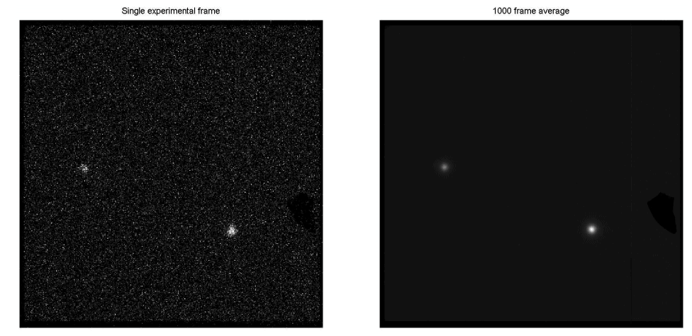
4.1 Experimental data
The experimental data consists of images of the field around the white dwarf g226-29 taken at 30 fps through a G filter. These data are presented in figure 2 and were gathered at the Mont-M´egantic observatory’s 1.6-m telescope at the f/8 prime focus. A stack of 1000 contiguous frames were used, consisting of 33 seconds of total integration time. The data was acquired with the first camera built with the CCD Controller for Counting Photons, and were first presented in [11]. The EM gain was set such that the effective readout noise of the system was 0.025 electron or alternatively, the EM gain over readout noise (G/σ) ratio was set to 40.
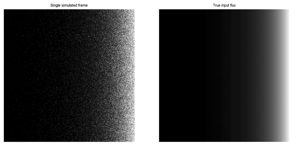
4.2 Simulated data
Simulated data were used to circumvent experimental biases or errors that could have contaminated the previous dataset. Experimental and simulated frames have identical dimensions. The latter present an input flux gradient on the horizontal direction: all pixels of a column share the same input flux and the input flux grows from the left to the right of the frame. Input fluxes were chosen so as to be uniformly distributed on a logarithmic scale on the interval from 10−2 to 101 photons per pixel per frame.
Various sources of EMCCD noise were modeled. Shot noise, thermal noise and CIC were generated from independent Poisson distributions. The ENF associated with the stochastic gain of the EM register was taken into account by a Gamma distribution. Finally, the readout noise was modeled as a zero-mean Gaussian distribution. Values for the dark noise (1 × 10⁻³ e/pixel/s at 67 frames/s) and CIC (0.001 e/pixel/frame) are taken from the Nüvü Camēras EM N2 512 EMCCD specification sheet [12]. The mean gain and readout noise were those of the experimental frames.
4.3 Frame window size
The question of how many sample frames should be considered to apply a post-processing method is important. Very often, these algorithms use statistical concepts requiring large sample sizes to reach reasonable accuracy. However, one must keep in mind that data remain limited in practice. Also, for real time applications, one may want to keep the window size small to get sufficient frame rate. The authors of [7] use N = 100 frames whereas the authors of [8] investigate the cases N = 5, 10, 20. While results of [8] show that the performance of their post-processing method increase with N for all input flux considered, the flux dependency does not seem to be influenced by the window size. Moreover, the performance gain is relatively small going from 10 to 20 frames (compared to going from 5 to 10 frames). Hence, willing to keep N small, this review uses a window size of 10 frames.
Having datasets containing 1000 frames, 100 groups of 10 frames are post-processed. Expression (5) is used to compute a NQE for each group. To assess the performance of a method, the averaged NQE of the 100 groups is plotted against the exact input flux. In the case of simulated frames, the exact flux S* is known for each pixel, while in the experimental case it is approximated by the mean raw signal s̅* taken over the 1000 frames.
One important thing to consider when comparing experimental and simulated curves in Figure 4 is the fact that the true flux S* is known and logarithmically distributed for simulated frames whereas it is unknown for experimental frames. This leads to a notable difference in the smoothness of the results as a function of flux. For simulated images, there is sufficient data in all flux bins from 10−2 to 101 photons per pixel per frame to accurately characterize the NQE. For experimental images, the “random” flux distribution of pixels does not permit an accurate depiction of NQE on all flux bins.
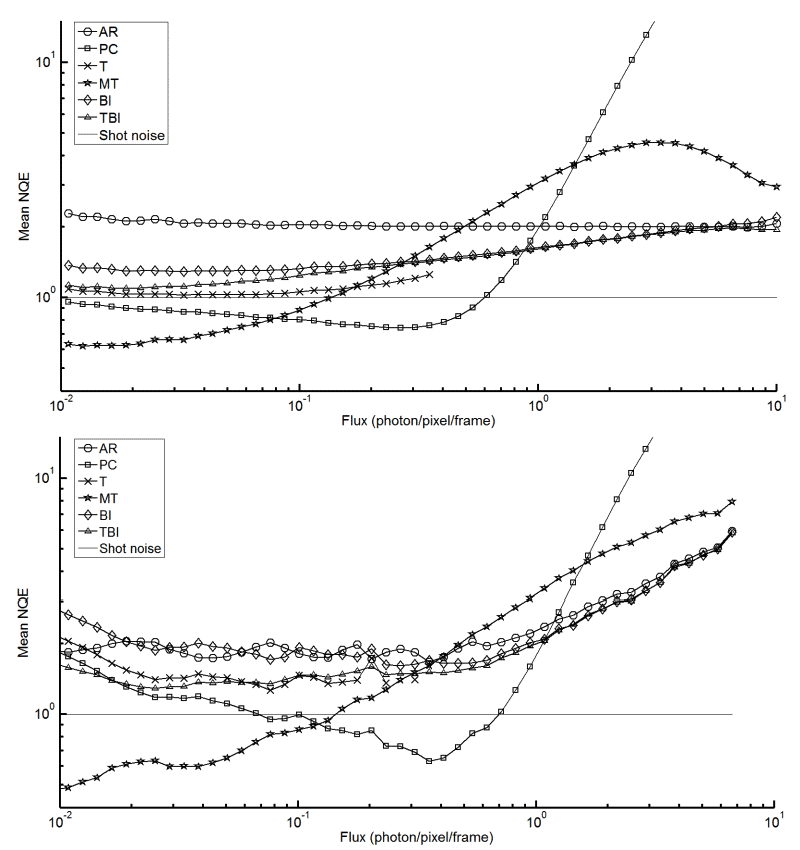
However, the meaningful aspect of this analysis is to show that both experimental and simulated curves have the same features so that a rigorous approach of EMCCD frame simulation and NQE comparison can be used to effectively assess the performance of EMCCD post-processing methods. With this in mind, both curves in Figure 4 give similar information in regards to the relative performance of different post-processing methods. This shows that using the NQE in combination with simulated frames is an optimal way to compare EMCCD post-processing methods. With the proposed optimized comparison method, Simulated Data of Figure 4 is used to give a general appreciation of EMCCD post-processing methods.
A feature to note in the flux behavior of the post-processing methods is the seeming “overshoot” of methods utilizing a thresholding scheme. These methods reach a maximum value of accuracy before diverging. In the studied flux ranges, MT accuracy dips erratically due to its non-linear photometric correction, PC diverges as it caps at 1 photon/pixel/frame and T diverges at increasingly lower flux ranges when the frame window size is reduced (frame window size dependency not shown). However, in experimenting with method parameters, it was noted that both BI and TBI exhibit this “overshoot” when photon flux approaches the maximum calculated values of their priors. It can be interpreted that this behavior is due to the maximum flux representation of each method.
Another feature of the NQE in Figure 4 is that PC and MT outperform the shot noise estimator of an idealized detector over bounded flux intervals. As mentioned in Section 2.1, the shot noise estimator is not an absolute lower bound for the NQE as it is not associated with perfect knowledge of the input flux. As a matter of fact, one could use a fictitious post-processing method that outputs 1 photon/pixel/frame independently of the camera output. This method would outperform the shot noise estimator around 1 photon/pixel/frame but would diverge for other fluxes. It would be unlikely that a method could take an EMCCD digital readout and be able to reproduce the true input flux for all input fluxes better than a detector that is only affected by shot noise. This is why an NQE that is more accurate than NQESN = 1 over a limited flux range is acceptable.
It is important to note that no method overcomes all others for all photon flux ranges. However, all the proposed algorithms outperform Analog Readout for extremely faint fluxes (_x001c_<< 1 photon/pixel/frame). This comes to no surprise as these post-processing methods are optimized for faint fluxes. One could be tempted to use a combination of multiple methods so as to maximize accuracy. However, as the true input flux is unknown in experimental situations, determining on which pixel to apply one method over another is a challenge to overcome.
In regards to proposing a systematic approach to comparing EMCCD post-processing methods, this article demonstrates that it is possible to use NQE combined with simulated frames to effectively assess the performance of EMCCD post-processing methods. For future research in this field, this method is suggested to compare postprocessing schemes.
During the study, it was observed that NQE performance of TBI and BI is very dependent on the values of k0. Choosing a value that is too low or close to the maximum flux value will result in a distortion of the NQE. Choosing a value that is too high will result in a dramatic increase of post-processing time. Thus the importance of choosing the value wisely.
If real-time performance is to be considered, the post-processing algorithm need to be looked at separately and fine-tuned. For future endeavors, an analysis of the effect of different post-processing parameters on the NQE curve aspect would be pertinent to test the robustness of this figure of merit.
1. P. Jerram, P. J. Pool, R. Bell, D. J. Burt, S. Bowring, S. Spencer, M. Hazelwood, I. Moody, N. Catlett, and P. S. Heyes, “The LLCCD: low-light imaging without the need for an intensifier,” in Sensors and Camera Systems for Scientific, Industrial, and Digital Photography Applications II, M. M. Blouke, J. Canosa, and N. Sampat, eds., Society of Photo-Optical Instrumentation Engineers (SPIE) Conference Series 4306, pp. 178–186, May 2001.
2. M. Stanford and B. Hadwen, “The noise performance of electron multiplying charge coupled devices,” IEEE Transactions on Electron Devices 1488R, Dec. 2002.
3. C. D. Mackay, R. N. Tubbs, R. Bell, D. J. Burt, P. Jerram, and I. Moody, “Subelectron read noise at mhz pixel rates,” 2001.
4. A. G. Basden, C. A.